Table of Contents
Example P20: Precipitation simulation during continuous casting of micro-alloyed Fe-Al-C-N-Nb-Ti steel, part 2: Precipitation kinetics in segregated and depleted regions
Compatibility
MatCalc version: 5.52.0034
Database: mc_fe.tdb, mc_x_FeAlCNNbTi.tdb, mc_sample_fe.ddb
Author: G. Stechauner
Created: 2011-11-29
Revisions: 2015-02-15 (P. Warczok)
Objectives
This is the second of two parts, which describe how to deal with primary precipitates. The method used in this example is thoroughly explained in the 'HowTo' manual for treatment of primary precipitates . The data from the transformation phases obtained in Scheil-Gulliver calculation are transfered into the precipitate phase and a calc state is created.
Part two utilizes this calc state. This is taken as the starting point for simulation of precipitation of TiN, NbC and AlN during cooling. As the liquid solidifies, a depleted and an enriched region will form due to segregation. Refer to the equilibrium example E20-4 - Scheil-Gulliver analysis of microsegregation if you want to test your knowledge on this topic. Using the chemical composition for the enriched and depleted regions, which is provided in E20-4, we can calculate the precipitation behavior in those extrema.
A discussion about the results will close this example.
Related documents
Complementary files
Click here to view the script for this tutorial.
Main document
Consider the same microalloyed steel as in example E20. Due to segregation a depleted region, as well as an enriched region forms. The chemical composition of C and N is assumed to be constant throughout the sample due to back-diffusion. The nominal composition is given in wt%.
| condition | C | Al | N | Nb | Ti |
|---|---|---|---|---|---|
| nominal | 0.22 | 0.025 | 0.0061 | 0.036 | 0.0081 |
| enriched | 0.22 | 0.014 | 0.0061 | 0.43 | 0.083 |
| depleted | 0.22 | 0.028 | 0.0061 | 0.0081 | 0.0021 |
Setup thermodynamics
Load the workspace file P20_1.mcw with the simulation results of part 1 or run the corresponding script to produce the results 'on the fly' (if your MatCalc version is elder than 5.61.1000 use the following script)
Setting up: Chemical composition, primary precipitates, heat treatment
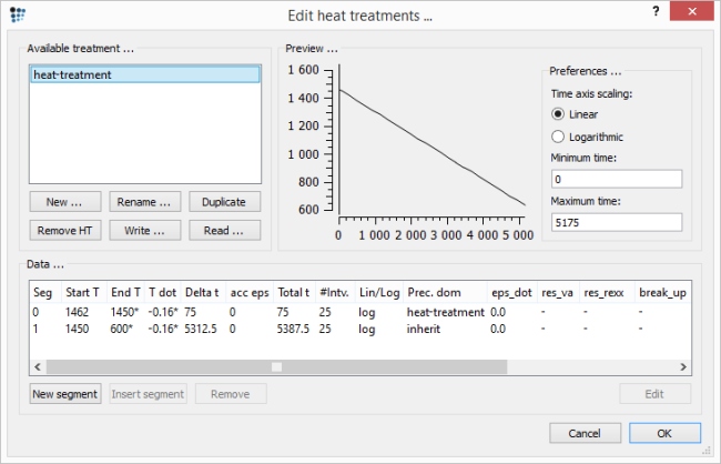
Obviously, as two regions with a different composition are to be investigated, there are two calculations which need to be performed. Before the start of each calculation, the system composition needs to be adjusted to the values given in the table above. Moreover, the primary precipitates which were created in the previous part of this example need to be introduced at the start of the simulation. But, before these issues are resolved, define the heat-treatment describing the cooling process as shown in the image below:
The opened 'p20-1.mcw' workspace has a stored calc state created at the end of the previous example part. This calc state contains the distribution of the primary precipitates which is the required input data for the simulations preformed in this part. Therefore, the heat treatment can be simply initialized from the calc state. However, the calc state itself contains also the composition of the system in which it was stored. For this reason it is necessary to load the calc state before the kinetic simulation, change the system composition and store it once again. This means that for the current example, two new calc states need to be created, each with the composition respective to the solute-enriched and -depleted region (with the according names, ideally). Then the simulation of each region is to be initialized from the coresponding 'new' calc state.
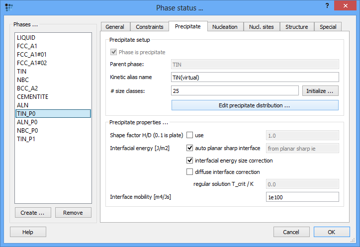
The more elegant solution would be the introduction of precipitate distribution from the file which was exported at the end of Example P20-1. This is the method of choice when the workspace with this precipitate distribution is not available (or cannot be opened by MatCalc for any reason). In order to simulate the condtion, when the precipitate distribution is not available, open the 'Phase status' window, select the 'TIN_P0' (this phase represents the primary precipitate), select the 'Precipitate' tab and click 'Initialize …' button. After accepting the question in the pop-up window, the phase will be re-initialized and all data on the distribution will be lost as promised. To import the data from the file, click on the 'Edit precipitate distribution …' button.
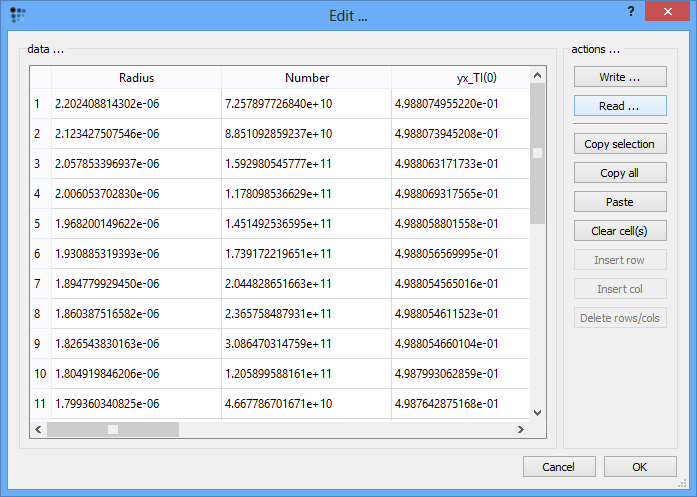
A new window opens which allows the edition of the precipitate distributions. After clicking on 'Read …' button, select the file 'size_dist_tin_primary.txt' to fill the empty cells with numbers.
Close the 'Edit …' window by clicking on 'OK' and accept the question about the application of the new data.
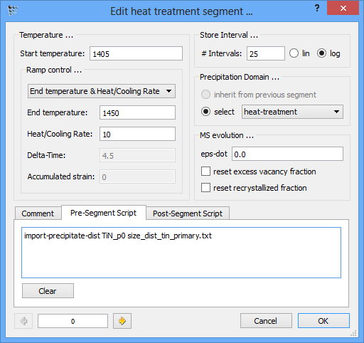
An alternative would be to use the console command
IMPORT_PRECIPITATE_DIST tin_p0 size_dist_tin_primary.txt
Type in this command into the pre-script of the very first segment in the 'heat-treatment' sequence.
Setting up the precipitation system and plots
To follow the growth of the precipitates during the heat treatment, a plot is needed. Create a p1 plot window with 4 plots and plot T$C, f_prec$*, num_prec$* and r_mean$*. Change the scaling and title of axes according to the figure below. Alternatively, run this script to set up the windows accordingly. Change the scaling type for the phase fraction to logarithmic and the scaling range to 1e-12..0,01.
Switch to the histogramm showing the number density over radius. In the options window on the sidebar, right-click on 'plot' and select 'new series - precipitate distribution'. Scroll down to the new series and select TIN_P0 as phase. Repeat this for the other three precipitates. Further change the scaling of the y-axis to logarithmic.
Starting the simulation
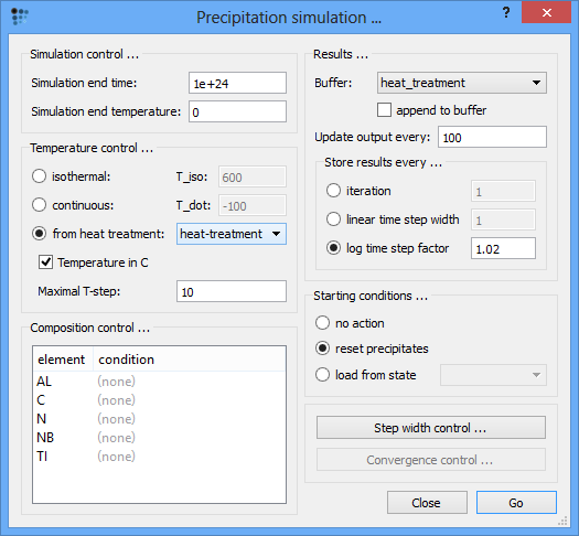
Enter the composition of the solute-enriched region. Next, bring up the 'Precipitation simulation …' dialog, and change the 'from heat treatment' setting to the properly configured 'heat-treatment'.
Press 'Go' to start the simulation.
Duplicate and lock the series, and repeat this step for the depleted calc state as well.
Result
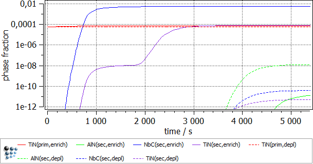
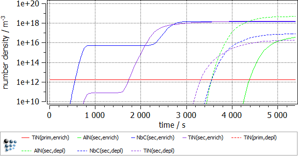
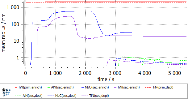
The following images show the result of this example.
As anticipated, the enriched region shows a higher phase fraction of TiN and NbC. It is interesting to note, that the precipitation of both the carbonitride phases occurs in 2 waves. The second burst of the precipitate results in the decrease of the mean radius value. AlN fraction is higher in the solute depleted region. This is due to the fact that the nitrogen supersaturation is higher there, as much less nitride precipitate is observed there. Lastly, some minor increase in the primary precipitate size was observed in the enriched region, due to the higher Ti concentration there.
Consecutive articles
none
