Table of Contents
Example P2: Precipitation sequence in Al-Cu, Part 1: Isothermal treatment of Al-Cu
Compatibility
MatCalc version: 5.50.0022
Database: mc_sample_al.tdb, mc_sample_al.ddb
Author: Georg Stechauner
Created: 2012-02-28
Revisions: Updated for 5.62.1000
Objectives
This example script simulates a technical Al-Cu alloy with 4.3 wt-% Cu. The script begins at high temperatures in the solution annealed condition where only the FCC_A1 matrix is present. Upon quenching to room temperature, precipitates form. Consequently the alloy is annealed at various temperatures isothermically. The size and phase fraction of precipitates will be plotted and discussed.
Related documents
Complementary files
Click here to view the script for this example for Version 5.62.1000 and newer. If it does not work with your MatCalc Version, check the older version of this script .
Main document
Setup thermodynamics
Use the mc_sample_al.tdb database for this example with the following elements, phases and chemical composition (given in wt-%):
| Elements | Composition | Phases |
|---|---|---|
| Al | ref. | FCC_A1 |
| Cu | 4.3 | THETA_AL2CU |
| - | - | THETA_PRIME |
| - | - | TH_DP_GPB |
Conclude the thermodynamic setup by reading the mc_sample_al.ddb diffusion database.
Precipitation domain and precipitates
The parameter set used in this example has shown to reproduce experiments considerably well. Feel free to use these values for your own simulations!
Open the precipitation domain window and create a new precipitation domain called 'almatrix'. Attach it to fcc_a1 phase. Enter the following value for shown settings:
| Tab | Option | Value |
|---|---|---|
| Structure | Grain diameter | 200e-6 |
| Dislocation density | 1e11 | |
| Vacancies | Consider excess vacancies | ✔, Enter 1 |
| Vacancy evolution model | FSK vacancy dynamics |
Be aware that the change performed at vacancies is of utmost importance. The FSK model is necessary for a more realistic vacancy dynamic. More on this factor and its influence later.
Follow by setting up the precipitates. Bring up the phase status dialog window and select the three Theta phases. Click 'Create new phase' and select 'precipitate'. This produces one precipitate phase for each of the selected phases. Enter the following commands to complete the system setup:
| Precipitate | Tab | Option | Value |
|---|---|---|---|
| THETA_AL2CU_p0 | Precipitate | #size classes | 25 |
| Shape factor | ✔, 0.1 | ||
| Nucleation | Nucleation sites | dislocations | |
| Nucleation constant | 0.01 | ||
| Special | Substitutional diffusion in precipitate as ratio from matrix | 0.1 | |
| Precipitate | Tab | Option | Value |
| THETA_PRIME_P0 | Precipitate | #size classes | 25 |
| Shape factor | ✔, 0.1 | ||
| Interfacial energy correction | 0.95*CIE$THETA_PRIME | ||
| Nucleation | Nucleation sites | dislocations | |
| Special | Substitutional diffusion in precipitate as ratio from matrix | 0.1 | |
| Precipitate | Tab | Option | Value |
| TH_DP_GPB_P0 | Precipitate | #size classes | 25 |
| Shape factor | ✔, 0.1 | ||
| Nucleation | Nucleation sites | bulk | |
| account for coherent misfit stress | ✔ | ||
| Structure | volumetric misfit | No flag, enter 0.03 | |
| Special | Substitutional diffusion in precipitate as ratio from matrix | 0.1 | |
| Excess vacancy trapping fraction | 0.002 |
Plots and diagrams
Proceed by setting up the output windows. Create a p1 plot and activate the default x-axis for all plots. Further change the title to 'Time [s]', scale the axis from '0.1..' and set its type to 'log'. Display the window in 2 columns.
Now create three new plots so you have four in total. Plot…
- …
T$Cin the first one. Change y-axis title to 'Temperature [°C]' - …
f_prec$*in the second one. Change y-axis type and title to logarithmic and 'Phase fraction', respectively. - …
r_mean$*in the third one. Change y-axis type and title to logarithmic and 'Mean radius [nm]', respectively. Change the factor on the y-axis to 1e9 to convert meters to nano-meters. - …
Num_prec$*in the fourth one. Change y-axis type and title to logarithmic and 'Number density [m-3]', respectively.
Defining the heat treatment
Even tough we are performing an isothermal heat treatment in this example, we need to start with rapid quenching, in order to nucleate the precipitates and to quench in excess vacancies. The influence of quenched in excess vacancies will be shown in this example, while the influence of quenching rate and other parameters will be shown in Part 2.
Open the 'Edit heat treatments…' dialog window and create a new heat treatment. Add a new segment and enter the following settings. Choose a starting temperature of 550°C and select 'almatrix' as the precipitation domain. Select 'inherit' for all following segments.
| Segment | Ramp control | End Temp. [C] | Cool. Rate [K/s] | Delta-Time |
|---|---|---|---|---|
| 0 | End Temp. & H/C Rate | 200 | 50 | - |
| 1 | H/C Rate & Delta Time | - | 0 | 1e9 |
Starting the calculation
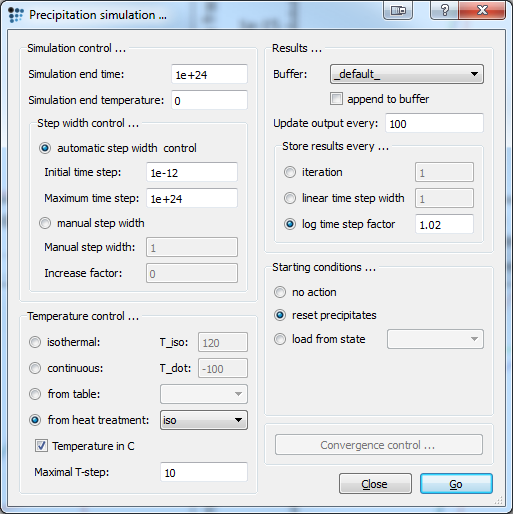
Start the simulation by opening the 'Precipitation simulation…' window and selecting the recently created heat treatment as 'Temperatur control'. Press Go to start the simulation.
In order to plot isothermal treatments at other temperatures as well, change the heat treatment and cool to other temperatures. Repeat the simulation then again.
Results: General
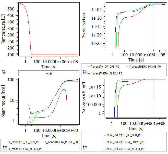
The result for an isothermal treatment at 150°C is shown below.
The results show a typical sequence for the given alloy. Upon cooling, at first the stable Theta phase nucleates, followed by the meta stable Theta_prime and Theta_double-prime. The influence of mean radius and number density on the evolution of phase fraction can clearly be seen. Only Theta_double-prime experiences an increase in number density after the nucleation, thus its increase in the phase fraction at about 10.000 seconds does not only root in the mean radius increase as for the other precipitates.
At about 1e7 seconds the meta-stable Theta_double-prime dissolves in favor of the stable Theta phase, which experiences another growth in mean radius after the small precipitates dissolved. The second meta-stable phase, Theta_prime does not dissolve in this example, as the annealing time is not long enough.
The next section will deal with different isothermal, annealing temperatures.
Results: Influence of vacancy model on phase fractions
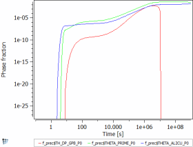
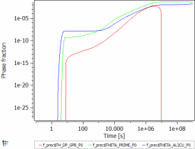
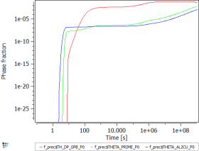
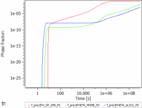
The figures below show the phase fractions and have been calculated with both the activated FSK model as well as no model. In order to deactivate the FSK model open the Precipitation domain window and switch to the vacancies tab. Select 'no vacancy annihilation/generation' instead of the FSK model and set 'no flag' at consider excess vacancies.
From the figures above the enormous influence of the FSK model on the precipitation behavior can easily be seen.
All temperatures show a difference in diffusion behavior, which gets more pronounced as the temperature of isothermal treatment decreases. While the curve progression of the 200°C figures is only slightly different when considering FSK-model compared to no vacancy annihilation/creation, a clear difference can be seen for the 100°C curve. A phase fraction of the first plateau of Theta_double-prime is obtained when considering the FSK-model about 3 orders of magnitude earlier than without the vacancy dynamics model.
The main reason for this temperature dependence is that the diffusion rate is still high at 200°C and therefore more or less independent of the excess vacancies. Moreover the diffusion correction factor due to non-equilibrium vacancy site fraction (XSV_DCF$almatrix) reaches its maximum at 20 and decreases in a few seconds to 1, where all the excess vacancies are annihilated again. For the 100°C the diffusion rate is slower overall. The correction factor raises to 1600 and needs 1000 seconds to reach unity again.
Note …
Consecutive articles
The analysis of this example will be continued in Part 2: Evolution of excess vacancies.
