Table of Contents
Example P30: Precipitation simulation in austenitic 316L steel: Evolution of Sigma, Chi and Laves precipitates
Compatibility
MatCalc version: 5.50.0022
Database: mc_x_FeCCrMnMoNiSi.tdb (alternatively: mc_fe.tdb), mc_fe.ddb
Author: Georg Stechauner
Created: 2012-06-19
Revisions:
Objectives
This example demonstrates the Simulation of the isothermal phase transformation of 316L at 815C, which was austenized at 1260C for 1.5h followed by water quench. The main interest of this example is the simultaneous nucleation of various phases at dislocations and grain boundaries.
Related documents
- B. Weiss, R. Stickler, Phase Instabilities During High Temperature Exposure of 316 Austenitic Stainless Steel, Metall Trans 3 (1972) 851-866.
Complementary files
Click here to view the script for this example.
Main document
Setup thermodynamics
Use 'mc_x_FeCCrMnMoNiSi.tdb' for this example with the following elements, phases and chemical composition (given in wt-%):
| Elements | Composition | Phases |
|---|---|---|
| Fe | ref. | FCC_A1 |
| C | 0.023 | M23C6 |
| Cr | 17.3 | Laves_Phase |
| Mn | 1.74 | Sigma |
| Mo | 2.66 | Chi_A12 |
| Ni | 13.1 | |
| Si | 0.73 |
Conclude the setup by reading the 'mc_fe.ddb' diffusion database. Afterwards, calculate an initial equilibrium at 1260°C - this is the start temperature of the kinetic simulation.
Precipitation domain and precipitates
The parameter set used in this example has shown to reproduce experiments, concerning austenitic steels, considerably well. Feel free to use these values for your own simulations!
Open the precipitation domain window and create a new precipitation domain called 'Austenite'. Attach it to 'fcc_a1' phase. Enter the following values for shown settings:
| Tab | Option | Value |
|---|---|---|
| General | Grain diameter | 400e-6 |
Follow by setting up the precipitates. Bring up the phase status dialog window and select the three Theta phases. Click 'Create new phase' and select 'precipitate'. This produces one precipitate phase for each of the selected phases. Enter the following commands to complete the system setup:
| Precipitate | Tab | Option | Value |
|---|---|---|---|
| M23C6_p0 | Nucleation | Nucleation sites | grain boundary |
| Precipitate | Tab | Option | Value |
| Chi_A12_p0 | Nucleation | Nucleation sites | dislocations |
| Precipitate | Tab | Option | Value |
| Sigma_p0 | Nucleation | Nucleation sites | grain boundary |
| Special | Diffusion in precipitate; from substitutional ratio | 1e-10 | |
| Precipitate | Tab | Option | Value |
| Laves_phase_p0 | Precipitate | Interfacial energy; auto planar sharp energy | remove ✔ |
| 0,73*CIE$LAVES_PHASE | |||
| Nucleation | Nucleation sites | dislocations |
Plots and diagrams
In this example, the four plots for precipitation kinetics will be created typical for precipitation kinetics simulation. These are:
- Temperature plot
- Displayed variable: T$C
- Y-axis title: 'Temperature [°C]'
- Phase fraction plot
- Displayed variable: F_PREC$*$WP → the unit qualifier “WP” in the suffix returns the phase fraction expressed in weight percent.
- Y-axis title: 'Phase fraction [wt.%]'
- Precipitate number density plot
- Displayed variable: NUM_PREC$*
- Y-axis title: 'Number density [m-3]'
- Y-axis type: log
- Precipitate mean radius plot
- Displayed variable: R_MEAN$*
- Y-axis title: 'Mean radius [nm]'
- Y-axis type: log
- Y-axis factor: 1e9
The x-axis, common for all plots is to be set up as following:
- Default x-axis for all plots: yes
- Default x-axis title: 'Time [h]'
- Default x-axis type: log
- Default x-axis scaling: 0,001..
- Default x-axis factor: 1/3600
Note: The making of the plots can be sped up by creation of the relevant user-defined plot window ('Create new window' → 'user-defined' tab). For this example, one can use the one called '03_kinetics_4_frames_T_f_n_r_logX' and modify it accordingly.
Defining the heat treatment
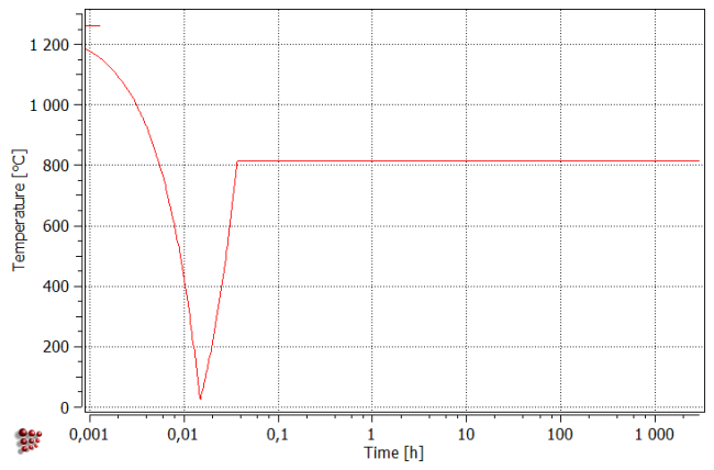
Even tough we are performing an isothermal heat treatment in this example, we need to start with rapid quenching, in order to nucleate the precipitates. It can be shown, that an isothermal treatment starting at 815°C without preceding quenching from solution temperature, results in no nucleation and growth of M23C6 precipitates. Keep this fact in mind, when designing isothermal heat treatments.
Open the 'Edit heat treatments…' dialog window and create a new heat treatment. Add a new segment and enter the following settings. Choose a starting temperature of 1260C and select 'austenite' as the precipitation domain. Select 'inherit' for all following segments.
| Segment | Ramp control | End Temp. [C] | Cool. Rate [K/s] | Delta-Time |
|---|---|---|---|---|
| 0 | End Temp. & H/C Rate | 25 | 23 | - |
| 1 | End Temp. & H/C Rate | 815 | 10 | - |
| 2 | H/C Rate & Delta Time | - | 0 | 3000*3600 |
Starting the calculation
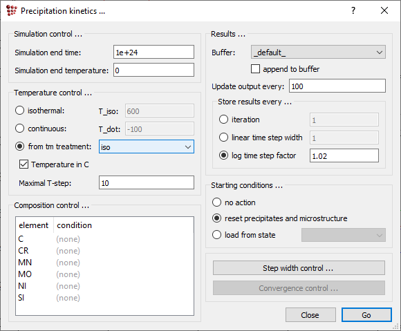
Start the simulation by opening the 'Precipitation simulation…' window and selecting the recently created heat treatment as 'Temperature control'. Press 'Go' to start the simulation.
Results: General
The result for the selected heat treatment Simulation are shown below:
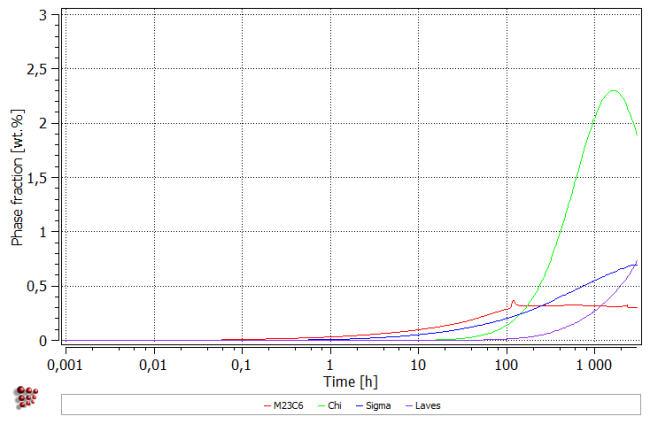
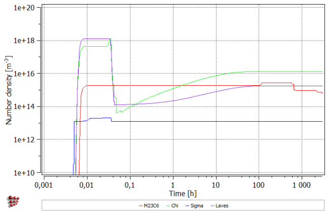
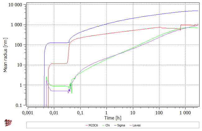
All precipitates appear during cooling to room temperature. Subsequent heating up results in the dissolution of the smallest precipitates of Chi an Laves phases (number density falls with the simultaneous increase of mean radius). During isothermal segment, all precipitates grow in size. Moreover, new precipitates of Chi and Laves phases appear within the first 100 hours. After about 1000 hours, Chi Phase decreases in size, resulting also in the fall of the phase fraction.
Results: Comparison to literature data
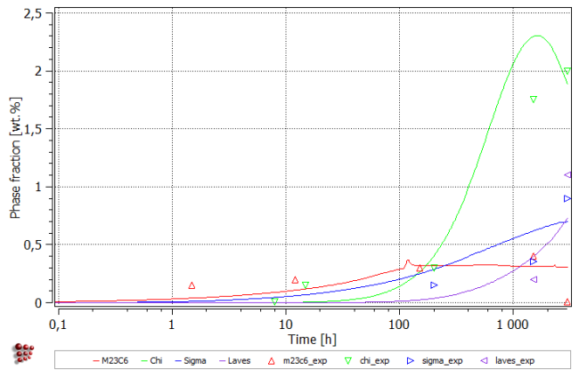
Create a table and enter following data to compare the calculated values to experimental ones:
| M23C6 | Sigma | Chi_A12 | Laves | ||||
|---|---|---|---|---|---|---|---|
| Time / s | wt-fraction | Time / s | wt-fraction | Time / s | wt-fraction | Time / s | wt-fraction |
| 10800000 | 0.0001 | 10800000 | 0.009 | 10800000 | 0.02 | 10800000 | 0.011 |
| 5400000 | 0.004 | 5400000 | 0.0035 | 5400000 | 0.0175 | 5400000 | 0.002 |
| 540000 | 0.003 | 720000 | 0.0015 | 720000 | 0.003 | ||
| 43200 | 0.002 | 0 | 0 | 54000 | 0.0015 | ||
| 5400 | 0.0015 | 0 | 0 | 28800 | 0.0001 | ||
Next, plot the table content on the phase fraction diagram.
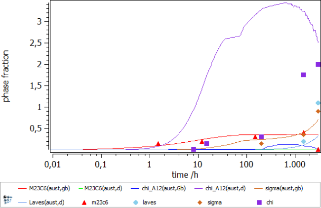
Simulation results are general in good agreement with the experimental data. The magnitudes of phase fractions are reproduced well. The amount of chi phase is decreasing towards the simulation end which is not confirmed with the experimental observation. On the other hand, the accuracy of the experimental data does not exclude such a scenario - an experimental investigation of the longer service times would help to resolve this question.
Further have a look at the following table, showing experimental versus calculated data of precipitate phases in respect to their chemical composition. To retrieve the simulated values, you can either plot the X$PhaseName$… variable or select the desired temperature in your buffer and read the data from the Phase details window.
| Sigma | Chi | Laves | M23C6 | |||||
|---|---|---|---|---|---|---|---|---|
| Exp. | Sim. | Exp. | Sim. | Exp. | Sim. | Exp. | Sim. | |
| %-Phase | 0.9 | 0.7 | 2.0 | 1.9 | 1.1 | 0.7 | traces | 0.3 |
| Mo | 11 | 23 | 22 | 19 | 45 | 40 | 14 | 21 |
| Cr | 29 | 24 | 21 | 24 | 11 | 15 | 63 | 72 |
| Fe | 55 | 41 | 52 | 49 | 38 | 39 | 18 | 7 |
| Ni | 5 | 12 | 5 | 8 | 6 | 6 | 5 | traces |
As before, the results are generally in good agreement to the experimental data. It is still ongoing work, to improve the thermodynamic description of phases, especially intermetallics as the sigma phase.
