MatCalc version: 6.0.0137
Database: mc_fe.tdb
Author: Yao Shan
Created: 2016-09-29
Revisions:

In this example, the basic features of the trapping kinetics is demonstrated. The site competition between sulphur and phosphor at grain boundaries will be highlighted in this simple example.

• Equilibrium trapping
• Trapping kinetics
• Example E30: Trapping in Fe-C
• Presentation of trapping model

Click here to view the script for this tutorial.

Create a new workspace and select the mc_fe.tdb as thermodynamic database for the example. For the elements select Fe, S and P. The example will only take one phase, BCC_A2, select this phase and read the database. Afterwards read the mc_fe.ddb diffusion database. For the composition take 0.5 wt% P and 0.5 wt% S. Afterwards calculate an equilibrium at 600°C.

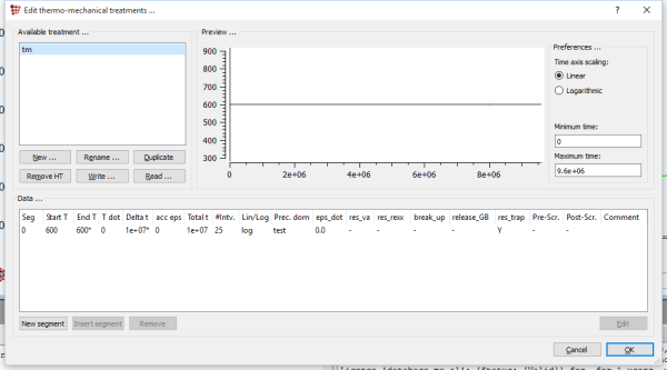
For the trapping kinetics to work, a thermomechanical treatment is necessary. Open the thermo-mech. treatment dialog from the Global menu or alternatively press Alt+F8. Here create a new treatment and give it a name (for example tm). Then create a new segment and double click onto it to start editing. Set the start temperature to 600. At ramp control select 'End temperature & Delta-Time'. Now you should be able to enter the end temperature of 600 and a delta-time of 1e7. Finally go to the MS Evolution tab and select the reset trap partitioning checkbox. Click OK to save the changes. Your treatment should now look similar to this

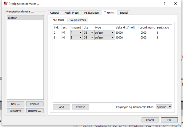
Open the precipitation domains dialog (Ctrl+F8) and create a new domain (name could be for example matrix). Then go to the trapping tab, you should now see blank table for FSK-traps. Click two times Add in the lower left corner to add 2 traps. In the trapped box select P for the first and S for the second trap. We want to trap S and P at grain boundaries, therefore select GB in the site box for each of the two traps. The type is default, which means it will apply the type shown in the lower right corner. This one is per default set to equilibrium. However, we want to do a kinetic simulation, thus, set the box to dynamic. Back to the traps, set the delta H value for the first trap to 30000 and the second to 10000. The coordination number is set to 1e4 for both traps. Now your dialog should look like this

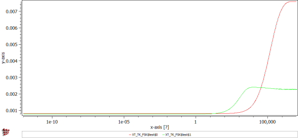
Create a new plot p1. In the variables window open the tab for prec_domain special. In here look for the XT_TK_FSK variable. This variable shows the mole fraction of an element which is trapped. Double click on the variable to open it and double click again on the variable one level lower to access the variables for the current precipitation domain. Here drag and drop the first two entries into the plot, which we created earlier. Finally click the x-axis in the plot and set the type to log in the options window.

Press Ctrl+K and select from tm treatment in the temperature control area. In the starting conditions select no action. Press go to start the simulation.