This tutorial was tested on
MatCalc version 6.02 rel 1.003
license: free
database: mc_fe.tdb

Click here to view the script for this tutorial.

• Adding further plots to a plot window
• Using the built-in variables
• Defining a default x-axis
• Modifying the series
• Adding a new series to a plot
• Removing a series from a plot
• Duplicating and locking series
• Editing series data
• Converting series to tables

Re-open the file saved in Tutorial 4 and save it under a new name.

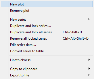
Highlight the plot window and right-click in this window outside the plot area to bring up the plot context menu already seen in Tutorial 4. Click on 'New plot'.

An empty plot appears below the original one.

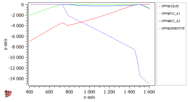
As well as the phase fraction variables 'F$*' encountered in the previous tutorial, MatCalc contains many other built-in variables which are evaluated at each step-value of the stepped equilibrium calculations. These can be found in the variables window. Information about each variable is contained in the small window below the main variables window. Locate the 'driving forces' category and drag 'DFM$*' to the empty plot window, to give a plot as shown below.

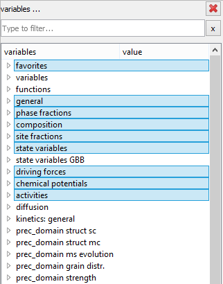
Other variable categories of particular interest for stepped equilibrium calculations are highlighted in blue in the image below:

This contains the most frequently needed variables: temperature in Kelvin ('T') and in Celsius ('T$C'), step-value, phase fractions ('F$*') and compositions expressed in mole fraction ('X$*$*') and in weight percent ('X$*$*$wp'). In these composition variables, the first asterisk represents the phase, and the second, the element, for example 'X$LIQUID$C'.

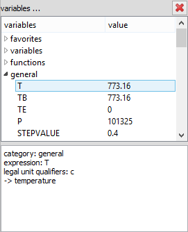
Temperature, step-value and pressure can also be found under this category. The temperature is in Kelvin by default, but the temperature in Celsius can be obtained by appending '$c', as has already been seen in the 'Favorites' category. This suffix is known as a 'unit qualifier'. Another unit qualifier is 'f' which appended to temperature variable in form of 't$f' returns the value of temperature in Fahrenheit. The 'information on variables' window shows the valid unit qualifiers for the variables:

The phase fractions 'F$*' are repeated here.

This contains the 'X$*$*' composition variables mentioned above, and a number of other composition-related variables, expressed either as either mole fractions (X…) or as u-fractions (U…). (Not all of these are applicable to stepped-equilibrium calculations, e.g. 'XPR$*$*' and 'UP$*$*' are for precipitation calculations).
Compositions in weight percent are not given separately here, but it can be seen from the 'variables information' window that 'wp' is a valid unit qualifier for the variables beginning with 'X'. This means that weight percentages can be obtained by appending '$wp' to the names of these variables.

The 'Y$*$*$*' variables give the site fraction of an element on a particular sublattice of a phase. For example, BCC_A2 has the variables 'Y$BCC_A2$FE$0' (site fraction of iron on sublattice 0) and 'Y$BCC_A2$C$1' (site fractions of carbon and vacancies on sublattice 1). The 'YX$*$*' variables represent the mole fraction of an element on a particular sublattice position of a phase; in this case, vacancies are not considered.

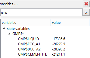
This category consists of a number of thermodynamic variables, including molar Gibbs free energies, entropies, enthalpies and heat capacities of the system and of each phase.

These categories include chemical potentials 'MU$*$*', activities 'AC$*$*' and activity coefficients 'ACC$*$*'.
Further plots can be added to the same plot window using 'New plot'; they will share the same buffer, default x-data and colour scheme. Some examples are shown below:

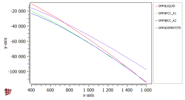
- Molar Gibbs free energy ('GMP$*')

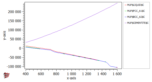
- Chemical potential of carbon ('MUP$*$C')

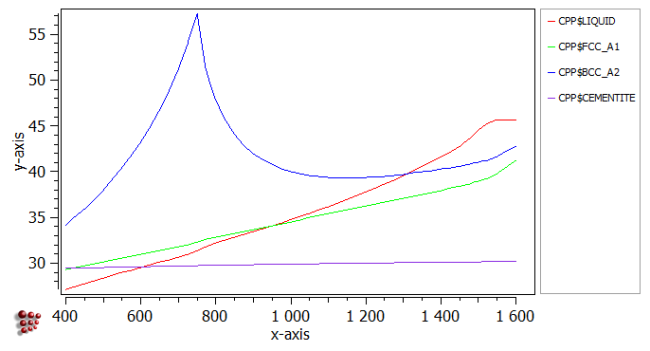
- Molar heat capacity ('CPP$*', note the lambda-anomaly at the Curie temperature in BCC_A2)

Note the search field on the top of the 'variables' window. By typing the variable name or a keyword (e.g. 'strength'), only the relevant variables will be shown.

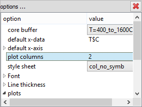
When there are many plots in the plot window then they will get streched so much that they will eventually become unreadable. In order to obtain a transparency, it might be a good idea to arrange the plots in more than one column. To place the plots in two columns, click on 'plot columns' in 'Options' window and type '2' in the appearing dialog.

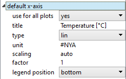
To give a consistent appearance to all the x-axes in the plot window, a 'default x-axis' can be defined. This is found towards the top of the 'Options' window. Change 'no' to 'yes' in the 'use for all plots' line and define the properties of the x-axis in the same way as for a normal x-axis.

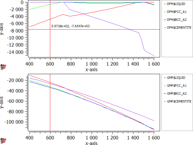
If the plot window contains several plots, right-clicking and dragging the mouse in one of these will display not only a cross in that plot, but a vertical line at the same x-value in all the others. An example is shown below:

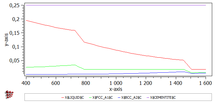
This part of the tutorial will demonstrate how to use the unit qualifiers mentioned above. Add a new plot to the plot window and drag and drop 'X$*$C' (carbon content of the phases) from the 'variables' window. The resulting plot should look like this:

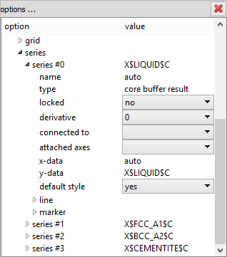
By default, the carbon content is expressed in mole fraction. To change the units to weight percent, firstly click on the new plot to select it. This should expand the section of the 'Options' list which applies to the new plot. Click on the triangle by 'series' to open the series options:

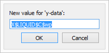
Double-click on 'y-data' for the first series to open the following box. Append '$wp' to the existing expression and click 'OK'.

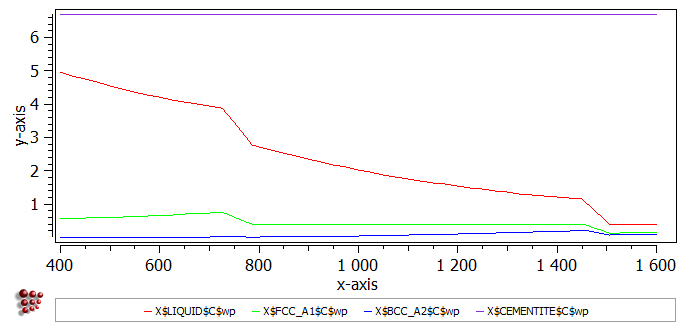
This will change the values plotted for the 'LIQUID' series. Repeat for the other three series. The final appearance of the plot, with appropriate axis labels added, should be as shown below.

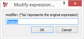
Alternatively you can select the variable and drag it to the window, and press 'Ctrl' before dropping it to the plot. An option window will pop up, where you can modify the original expression (read as %s) by adding mathematical operations or change it to weight percent by appending '$wp'.

Note: Press 'Ctrl'-key after selecting in 'variables' window and before dragging the desired variable.

Right-clicking on 'series' in the 'Options' window displays a context menu:

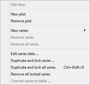
The 'New series' part of the menu expands to give the following sub-menu (provided that a plot is selected).

Clicking on 'core buffer results' creates an empty series (given the name of 'auto' on the plot) to contain variables evaluated from the results of a buffer. Edit the 'y-data' line in the 'Options' window for this series to enter any valid built-in or user-defined variable or an expression.

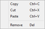
Variables can be copied from the 'Variables' window by right-clicking on the expression required to display a menu containing Copy, Paste and other operations.

The other series types which can be added are as follows:

- 'table/experimental data': allows the user to add a set of experimental data points to a plot. This will be demonstrated in Tutorial 10
- 'function/expression': enables an algebraic expression in (x) to be entered. This will be demonstrated in Tutorial 12

To remove a series from a plot, first click on the plot to select it. This will expand the part of the Options list which applies to the plot. Select the name of the series from this list and choose 'Remove series' from the right-click menu (shown above) or press 'Delete'. Multiple series in the same plot can be selected at once by holding down the CTRL key while clicking on the series names. 'Remove all series' in the right-click menu deletes all the series in the selected plot. 'Remove all locked series' removes all the series which are locked (locking the series is described below).

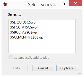
This feature is available in the right-click menus of both the Options window and the plot window. Click on 'Duplicate and lock series', select a series from the list shown and click on 'Duplicate' button. This will lock the original series and create a copy.

'Duplicate and lock all series' performs this operation for all series in the selected plot window.

The locked series is protected from any changes when the buffer contents are updated with new calculation results, while the copy is unlocked. This enables an easy comparison between results obtained under different conditions.

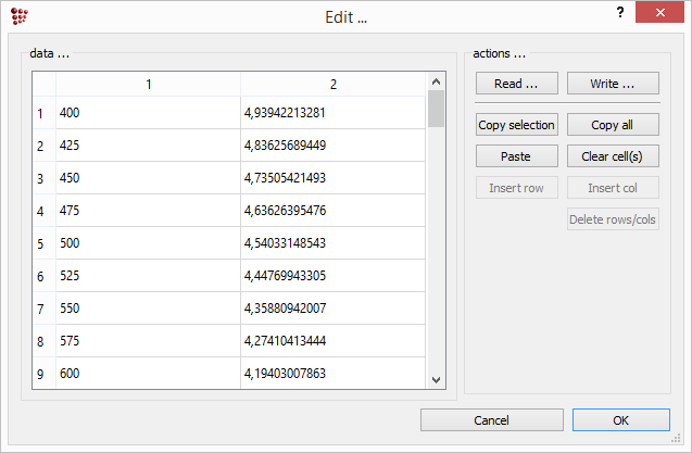
This is also available in both the Options and the plot windows. Select a series in the appearing window and click on 'Edit…' to display a table containing the numerical data used to plot the graph.

The data can be copied using the 'Copy selection' or 'Copy all' buttons. The contents of the rows and columns can be modified using 'Paste' (to add data copied from another source), 'Clear cell(s)', 'Insert row', 'Insert col' and 'Delete rows/cols' buttons. Use 'Write' to save the whole dataset to a text file and 'Read' to load a dataset from a text file.

This places the data from the series into a named table, which can be accessed from the 'Global' menu.
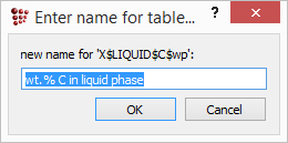
Select the 'series' in 'Options' window, click on 'Convert series to table', select the series name and edit the name of the table, if necessary, in the box which appears, as shown below.

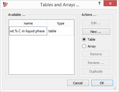
To open and edit a table, select 'Tables and arrays' from the 'Global' menu. This will display a list of all the available tables, which can be edited in the same way as the series data described above.

The tutorial is continued in article T6 - Introduction to user-defined functions.

Go to MatCalc tutorial index.