This tutorial was tested on
MatCalc version 6.04 rel 1.001
license: free
database: mc_fe.tdb

Click here to view the script for this tutorial.

• Creating a new graphical window
• Introduction to the variables window
• Modifying the appearance of a plot using 'options'
• Zooming in and displaying x- and y-values
• Exporting a plot as an image and as numerical data

Open the file saved from Tutorial 3 and select the buffer named 'T=400 to 1600°C'.

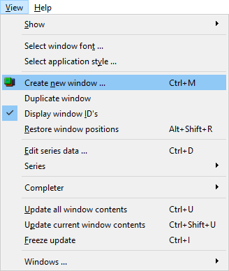
To plot numerical results, it is first necessary to create a graphical window. In the 'View' menu, click on 'Create new window' or click on icon.

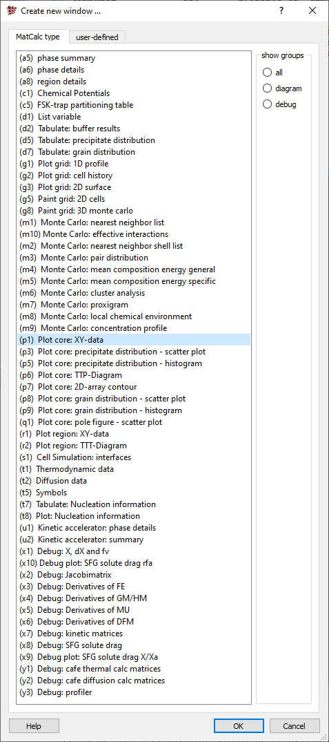
In the 'Create new window' box which appears, there is a list of a number of possible window types. Among these are '(a5)' and '(a6)', which are the familiar 'phase summary' and 'phase details' windows automatically placed on the screen when a new workspace file is created.
Select type '(p1) Plot core: XY-data' and click on 'OK'

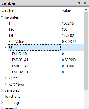
An empty plot with x- and y-axes appears on the screen. Locate the 'Variables' window - if it is not present, right-click in the toolbar area at the top of the screen and select it from the menu, or click on icon in the 'Quick Access' menu. Expand the 'favorites' section by clicking on the small plus-sign to its left. Then, further expand the section labelled 'F$*' to give the list shown below.

The syntax 'F$BCC_A2' means 'the phase fraction of BCC_A2', where the dollar sign is a separator between the variable 'F' and the phase to which it applies 'BCC_A2'. In the heading of the list, 'F$*', the asterisk is a wild-card indicating 'all phases'. The meaning of the variable symbols can be found in the 'information on variables' part of the 'variables' window (see Tutorial 1). Select 'F$*', drag it to the empty plot and drop it.
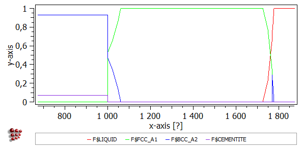
The plot should appear as shown below:

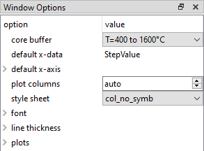
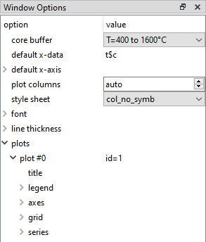
The 'Options' window can now be used to modify the appearance of the plot as required. (Again, if this is not currently shown, it can be made to appear by clicking on icon in the Quick Access menu or the right-click menu in the toolbar area.)

Firstly, note that there is a 'buffer' drop-box. By selecting one of the other buffers, the contents of the plot can be changed. The 'default x-data' option (the second line down in the options window) is set to StepValue, i.e. the value of the stepped variable used in the stepped equilibrium calculation.
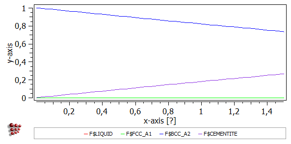
Thus, on selecting the 'C=0 to 1.5 at 500°C' buffer, the x-value changes to carbon content, and the plot looks like this:

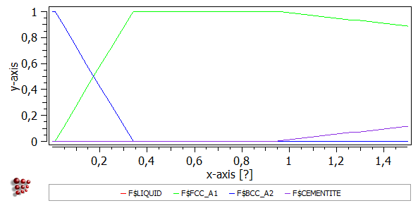
and the plot for the 'C=0 to 1.5 at 800°C' buffer looks like this:

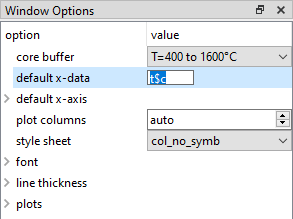
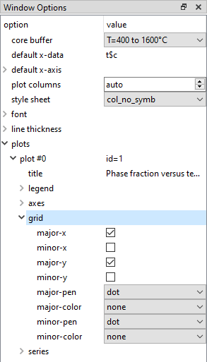
Select the 'T=400 to 1600°C' buffer from the buffer drop-box. One of the first things to note is that the x-axis data does not run from 400 to 1600; this is because the step value is expressed by default in Kelvin rather than in Celsius. To change this, double-click on the 'StepValue' text in 'default x-data' line. Enter 't$c' (temperature in Celsius) in place of 'StepValue'.

The plot can be changed from colour to black-and-white ('b/w') using the 'style sheet' drop box.
The 'plots' section of the options menu can be expanded by clicking on the white triangle. Below 'plot#0' (the name of the current plot) is a list of options for this plot:

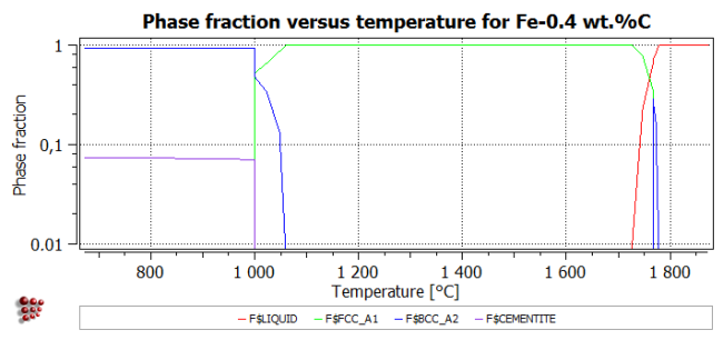
This is blank by default. Double-click to enter a title, e.g. 'Phase fraction versus temperature for Fe-0.4 wt.%C'.

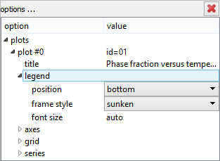
This comprises options for the position of the legend and for the style of the box surrounding it. In field 'position' change the setting to 'bottom'

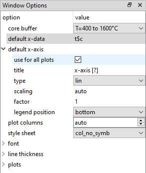
One might wonder, why the legend was shown from the start in the bottom, while the original setting was set to 'right'. It is because the changes on the legend properties will be visible only when the 'use for all plots' box at 'default x-axis' is checkmarked. More information about the 'default x-axis' concept will be given in the next tutorial.

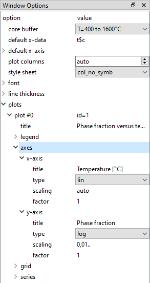
The 'axes' section expands to give options for the 'x-axis' and 'y-axis'.

Double-clicking on the 'title' line for x-axis will bring up a box entitled 'New value for 'title':'. Enter 'Temperature [°C]'. In the same way, change the y-axis title to 'Phase fraction'.
The axis type can be set to either linear or logarithmic. A linear scale is more suitable for the temperature axis, but a logarithmic y-axis enables the fractions of minor phases, such as cementite in this example, to be seen more clearly. Change 'lin' to 'log' for the y-axis.
The automatically assigned minimum y-value on the log-scale may not be appropriate, so if this is the case, double-click on 'scaling' and replace 'auto' with '0.01..1'. The two numbers are the lower and upper limits respectively. If one or other of these is missed off, an automatic value is assigned instead. (For example, using '0.01..' is sufficient to give a scale from 0.01 to 1, since 1 is the maximum value of F$*).
The changes on the x-axis properties will be visible only when the 'use for all plots' setting at 'default x-axis' is set to 'no'.

This allows gridlines to be added to the plot, and their appearance to be modified. Change 'disabled' to 'enabled' for 'major-x' and 'major-y' to show major gridlines.

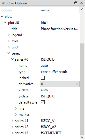
Expanding the 'series' section gives a list of options for each data-series. The name of the series (as it appears in the legend) can be changed using 'name'.
The 'locked' option, when set to 'yes', protects the series from any changes when the contents of the buffer are updated. A locked series is indicated by an asterisk by the name, if the automatic name is used.
'Derivative' can be used to display the numerically evaluated first or second derivative of a series.
The 'x-data' and 'y-data' options control which data-sets are displayed on the x- and y-axes. If the 'x-data' is set to 'auto', the default x-data, as specified above, is used.
The appearance of the plots can be modified by setting 'default style' to 'no' rather than 'yes', and then expanding 'line' and 'marker' to give a list of options for colours, styles, sizes etc.

The image below gives an example of a modified plot.

Left-click in the plot area and drag the mouse to draw a rectangular box. When the mouse button is released, an enlarged version of the region within the box is shown on the axes. Right-click anywhere in the plot area to return to the original scale.

When moving the mouse pointer on the plot area, a black cross appears with the y- and x-values next to it. The coordinates of the centre of the cross are also shown on the status bar at the bottom left of the screen. A larger, red cross can be obtained by pressing the right mouse button.

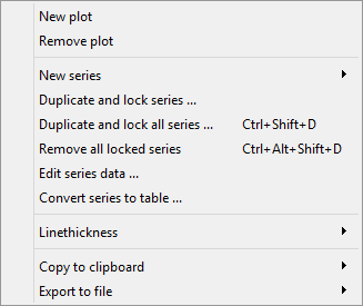
Right-clicking in the plot window but outside the area of the plot itself gives a context menu as shown below.

Clicking on 'Copy to clipboard' allows to export this single plot or the whole frame (i.e. all plots in this window) in the pixmap (.bmp) or scalar vector graphics (.svg) format. Then the exported piece can be pasted to the relevant graphical application. Additional for the plot, there is a possibility to export the numerical data which will appear in the form of tab-separated columns after the paste operation.
Clicking on the 'Export to file' will create the file containing the plot or the whole frame. The possible output file formats are '.png', '.svg' and '.pdf'

Save the workspace file.

The tutorial is continued in article T5 - MatCalc built-in variables; graphical output

Go to MatCalc tutorial index.