This tutorial was tested on
MatCalc version 6.04 rel 1.002
license: free
database: mc_fe.tdb; mc_fe.ddb

Click here to view the script for this tutorial.

• setting up a simulation grid
• assigning properties to cells
• setting up display of cell simulation results
• setting up simulation parameters
• boundary conditions

MatCalc can be used to carry out simulations of long-range diffusion problems, and problems in which diffusion is coupled with precipitation, using a finite-element method with the system divided into a number of cells. Many examples of the application of this functionality, in different systems and with different boundary conditions, can be found in the relevant part of the 'Examples' section. The present tutorial demonstrates a simple case for which an analytical solution of Fick’s 2nd Law is available. The numerical and analytical solutions are compared.

The functionality for setting up and running diffusion simulations is only available through the scripting language and not through the GUI. This tutorial therefore also serves as a refresher for some of the basic scripting commands that we have already encountered, as well as introducing the new commands needed to set up and run diffusion simulations.

Fick's Second Law of Diffusion is a partial differential equation of the form:

\[ \left({\partial C \over \partial t}\right) = D . \left({\partial^2 C \over \partial x^2}\right) \]

where $D$ is the diffusion coefficient, which is here assumed to be independent of concentration. This equation can be solved to give the concentration $C$ of the diffusing species as a function of distance $x$ and time $t$. The form of the solution depends on the boundary conditions. In most cases, a numerical solution using finite-difference or finite-element methods is required, but there are some special cases in which an analytical solution is also available.

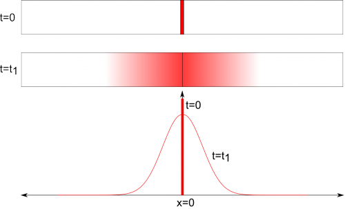
One of these is the thin-film solution, in which an very thin layer containing a finite amount of the diffusing species is sandwiched between two semi-infinite bars of material. The boundary conditions are that:

• initially, the concentration of the solute in the bar is zero; this is expressed mathematically as $ C\{x=0,t=0\}=0$ , where $x$ is the distance from the midpoint marked by the central black vertical line in the diagram below, and

• the total amount of solute is finite and constant throughout the time period considered; this is expressed mathematically as

\[\int_{-\infty}^{\infty} C \{x,t\} \mathrm{d}x = B,\] where $B$ represents the amount of solute in the system.

The standard solution when the boundary conditions are of this type is of Gaussian form:

\[ C\{x,t\} = {B \over 2 \sqrt{\pi D t}} . \mathrm{exp}\left({-x^2 \over 4 D t}\right) \]

In this tutorial, we will set up a cell-based numerical simulation of a situation that fulfils these conditions to a reasonably good approximation, i.e. a thin layer of FCC iron with a relatively high carbon content sandwiched between two bars of FCC iron with a very low carbon content. The results of this simulation will be compared with those obtained using the analytical solution.

Start MatCalc and create a new script file as explained in Tutorial 13.

The first task that the script must perform is to create a new MatCalc workspace. Type the following command into your script window:

use-module core

This tells MatCalc to use the core module, which it selects at the begining by default anyway; later in this tutorial we will see the use of the simulation module.

new-workspace 

This creates a new workspace. If an existing unsaved workspace is open when the script is run, you will be prompted to save it. To disable this prompt, append f to the new-workspace command.

Some workspace information can be added as shown:

@$************************************
$ enter workspace info
@$************************************
@ set-workspace-info Script T23
@ set-workspace-info +Simulation of long-range diffusion of C
@ set-workspace-info +out of thin film
@ set-workspace-info +with matrix phase FCC_A1.

The next step is to set up the thermodynamic and kinetic data. Enter the following commands into your script window and save the script.

open-thermodyn-database mc_fe.tdb
select-elements fe c
select-phases FCC_A1
read-thermodyn-database
read-mobility-database mc_fe.ddb

Following this, define the variables that will specify the initial carbon content in the bar (c_comp_bar_wp) and the thin layer (c_comp_layer_wp) so that these can be used later. Note that the carbon content of the bar is set to be very low, but for numerical reasons it is not advisable to set this to exactly zero.

set-variable-value c_comp_bar_wp 1e-10
set-variable-value c_comp_layer_wp 0.8

In the cell simulation, compositions must be entered in molar notation un$c. The code below enables you to enter a composition in weight percent (wp) and then save the composition in mole fraction as a variable for use in the cell simulation.

enter-composition wp c=c_comp_bar_wp
set-variable-value c_comp_bar un$c
enter-composition wp c=c_comp_layer_wp
set-variable-value c_comp_layer un$c

Then set a temperature and calculate an equilibrium to initialise the system and check that everything is working OK.

set-temperature-celsius 1000
calculate-equilibrium

At this stage, also specify the simulation time (in seconds) for subsequent use:

set-variable-value sim_time 1e7

Save the script. It is recommended to test it out at this stage to catch any typing errors before going further.

Before setting up the cell simulation, you must define a precipitation domain, i.e. a matrix of phase FCC_A1; this is necessary for subsequent use in the cell simulation.

create-precipitation-domain aus_domain
set-precipitation-parameter aus_domain X FCC_A1 

The next step is to set up the cell simulation. First change to the simulation module:

use-module simulation

Define a variable representing the number of cells:

set-variable-value num_cells_x 99

Then create a simulation grid using the command:

create-simulation-grid num_cells_x 1 1 

The three numbers here represent the number of cells in the x-, y- and z-directions, respectively. Define a variable representing the length of the bar:

set-variable-value barlength 0.099

Specify the dimensions in these directions (in m) using the command:

set-grid-coordinates barlength 1 1 

and the geometry of the grid, using the command:

set-grid-geometry p 

The three geometry options are:

• p - planar
• c - cylindrical
• s - spherical

To visualise this grid, create a new window of the type g5 (Paint grid: 2D cells):

new-gui-window g5

Give this window a name so that it can be referred to easily later. The variable active_frame_id used here is one of MatCalc's internal variables; see the section of the Reference book on internal variables for details.

set-variable-value paint_window_id active_frame_id 

Modify the position, size and zoom level using the following two commands:

move-gui-window paint_window_id 0 100 750 160 $ change position and size
set-gui-window-property paint_window_id i Z 200 $ zoom 200%

The grid should now look as shown:

In the next section, properties will be assigned to the cells in the grid.

For the diffusion simulation, it is necessary to create a material and assign to this the precipitation domain called aus_domain that was created above:

create-material aus_material
set-material-property aus_material G D aus_domain 
$ [g]eneral properties: [d]omain

Then set the diffusion coefficient. Here, a user-specified value is used, instead of one calculated using information from the database, to better facilitate comparison with the analytical solution. The diffusion coefficient is stored in a variable for later use. The syntax below means [d]iffusion [c]oefficient of [c]arbon, [f]unction or expression.

set-variable-value diffCoeff 1e-12
set-material-property aus_material D C C F diffCoeff
$[d]iffusion [c]oefficient of [c]arbon, [f]unction or expression

Following this, assign properties to the cells. Using the syntax below, the material aus_material is attached to all the cells.

set-cell-property a m aus_material $[a]ll cells, [m]aterial

Set the temperature of all cells to 1000˚C, by first specifying that the temperatures should be in ˚C:

set-simulation-parameter N Y

specifying the temperature in the form of a variable:

set-variable-value sim_temp 1000

and then attaching this temperature property to all cells:

set-cell-property a V T sim_temp $ [a]ll cells, [v]ariable, [t]emperature

Assign the lower carbon content, c_comp_bar, to all cells.

set-cell-property a V C C c_comp_bar 
$ [a]ll cells, [v]ariable, [c]omposition [c]arbon

The next stage is to select the cell in the middle of the bar using its cell index. First, we note that the first cell has the index 0, so the highest cell index in the array obtained using:

set-variable-value max_cell_index num_cells_x-1

and the index of the cell in the middle is given by:

set-variable-value middle_cell_index max_cell_index/2

Then select the cell in the centre by its c[e]ll index:

add-cell-selection E middle_cell_index $ select the cell in the centre.

Assign the higher carbon content, c_comp_layer, to the selected cell (denoted by an asterisk).

set-cell-property * V C C c_comp_layer 

The g5 window shows, by default, the selected cell(s) in blue:

The next stage is to set up the graphical display to look at the results. Firstly, assign a property to the existing paint window created above, paint_window_id so that the cells are coloured according to their carbon content.

set-gui-window-property paint_window_id I W V $ display cell variable
set-gui-window-property paint_window_id I V _cwp$c $ set which variable
set-gui-window-property paint_window_id I R 0..1

In the first line in the code above, the syntax represents s[i]mulation results, display [w]hat, [v]ariable. In the second, the [v]ariable is specified as _cwp$c, and in the third, the [r]ange is specified. The variable syntax _cwp$c represents the set of values of wp$c (weight percent of carbon) in the cells. Variables of this type can be found in the variables window under cafe: cells.

The cell array is shown schematically below, where blue represents a lower carbon content, and yellow a higher.

In addition, make a profile plot of the carbon content. Create a window of type g1: plot grid: 1D profile.

new-gui-window g1

Assign a name to both the plot window and the plot itself:

set-variable-value profile_window_id active_frame_id 
set-variable-value profile_plot_id last_plot_id 

Add a [s]eries, [n]ew of the [s]imulation variable _cwp$c.

set-plot-option profile_plot_id S N S _cwp$c

Specify that the default x-axis should be used, and give it a title:

set-gui-window-property profile_window_id S U Y 
set-gui-window-property profile_window_id S T Position [m]

Label the y-axis and specify its range:

set-plot-option profile_plot_id A Y 1 T Carbon content [wt.%]
set-plot-option profile_plot_id A Y 1 S 0..c_comp_layer_wp 

Give the plotted series the name 'Numerical':

set-plot-option profile_plot_id S M 0 Numerical 

Specify the range of cells over which the profile is to be taken. In the syntax here, the first line gives the index of the s[t]arting cell (here 0) and the second line gives the index of the st[o]p cell (here max_cell_index).

set-gui-window-property profile_window_id I t 0
set-gui-window-property profile_window_id I o max_cell_index

Give the window an appropriate size:

move-gui-window profile_window_id 20 20 600 400

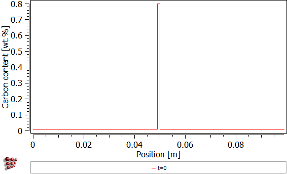
The plot should look as shown:

We will now create a third window to display the time-dependent evolution of the carbon concentration in selected cells. The required window type is g2: Plot grid: cell history. Create the window and assign a name to the window and plot.

new-gui-window g2
set-variable-value history_window_id active_frame_id 
set-variable-value history_plot_id last_plot_id 

Use the following commands to specify that the default x-axis should be used and to assign it a title and a range.

set-gui-window-property history_window_id S U Y  $use default x-axis
set-gui-window-property history_window_id S T Time [s]
set-gui-window-property history_window_id S S 0..sim_time 

Label the y-axis and specify its range:

set-plot-option history_plot_id A Y 1 T Carbon content [wt.%]
set-plot-option history_plot_id A Y 1 S 0..c_comp_layer_wp 

Now add two series, firstly the composition of the middle cell, and then that of the cell adjacent to it.

set-plot-option history_plot_id S N S _cwp$c{middle_cell_index}
set-plot-option history_plot_id S N S _cwp$c{middle_cell_index-1}

Give these series titles. Note that the quotation marks are needed for a multi-word title, as in the case of the series 'next to centre'

set-plot-option history_plot_id S M 0 centre 
set-plot-option history_plot_id S M 1 'next to centre'  

Finally, resize and move the history plot.

move-gui-window history_window_id 800 20 600 400

In the final stage before setting up and running the simulation, the analytical solution will be added to the existing profile plot. Since the expression is rather complicated, it will be divided up into simpler terms:

Bval*term_1*term_2

where Bval represents the integral giving the amount of solute in the system:

\[B = \int_{-\infty}^{\infty} C \{x,t\} \mathrm{d}x,\]

term_1 is the term

\[ {1 \over 2 \sqrt{\pi D t}} \]

and term_2 is the term

\[ \mathrm{exp}\left({-x^2 \over 4 D t}\right) \]

The value of the term $B$ can be estimated by assuming that the initial concentration of carbon in the bar is small enough to be neglected, such that initially all the carbon is in the layer in the middle of the bar. The value of $B$ is then simply the carbon concentration in the layer (in the units in which the curve is to be plotted, here weight percent, c_comp_layer_wp), multiplied by the width of the layer. The layer is one cell wide, i.e. the bar length divided by the number of cells.

set-variable-value Bval c_comp_layer_wp*(barlength/num_cells_x)

The cell variables (prefixed with _c) that we have seen earlier in this tutorial can be included in variables and functions. For example, term_1 uses the cell variable _ctime to represent the time in the cell simulation. The variable diffCoeff was defined above, and pi is a built-in variable. (For details of the built-in variables of MatCalc, consult the section of the Reference Book on internal variables.)

set-function-expression term_1 1/(2*sqrt(pi*diffCoeff*_ctime))

It should be noted that the term x in the mathematical formulation of the analytical expression is measured from the centre of the range, whereas the cell variable corresponding to the x-position of the centre of the cells, _ccenter_x, is measured from the left-hand side of the system. We must therefore create an expression for the shifted x-coordinate:

set-variable-value midpt barlength/2
set-function-expression x_shifted _ccenter_x-midpt
set-function-expression term_2 exp((-1*x_shifted**2)/(4*diffCoeff*_ctime))

The analytical expression is then given by:

set-function-expression analytical_expr Bval*term_1*term_2

and this series is plotted onto the existing profile plot using the command:

set-plot-option profile_plot_id S N F analytical_expr 0..barlength

The 0..barlength expression in the command above represents the range over which the function is to be evaluated; this corresponds to the length of the bar.

Note that when the analytical expression is first plotted, it looks slightly strange. This is because the time is initially zero, leading to a value of zero in the denominator of the first term, term_1.

The final set of commands deals with the simulation time and temperature, boundary conditions, type of simulation and update interval.

set-simulation-parameter e sim_time $ end

Specify the update interval:

set-simulation-parameter u 10 $ update interval

It is now necessary to tell the simulation module what type of problem should be simulated, i.e. how temperature and diffusion should be treated. In this case, we wish to simulate a diffusion-field problem, in which the elements are allowed to diffuse through the system:

set-simulation-parameter d f $ diffusion-field simulation

The temperature control, by contrast, is set to be isothermal and the hold temperature specified in terms of the variable sim_temp set earlier.

set-simulation-parameter t i sim_temp $ temperature: isothermal

The final step is to set up the default boundary conditions, i.e. the boundary conditions that apply in the absence of any other boundary conditions being set for specific cells or groups of cells. The type of boundary condition required is [g]eometric, and is set to [o]pen to environment. This means that there is no periodicity or symmetry.

set-default-boundary-cond G O $ open to environment.

Save the script.

To run the script, click on Script > Run Script, press Shift + F2 or click on the button. Then select the name of the script you wish to run from the drop-down menu and click on Go.

When the script has been correctly executed, select Simulation > Start simulation or press Ctrl + J to start the simulation. Output will appear in the Console, starting with:

#####################################################################

 starting microstructure simulation ...

#####################################################################

and finishing with:

####################################################################################################


microstructure simulation finished in 59.07 secs (tot 59.07 secs) on Fri, 2016-06-10, 17:57:34 


####################################################################################################

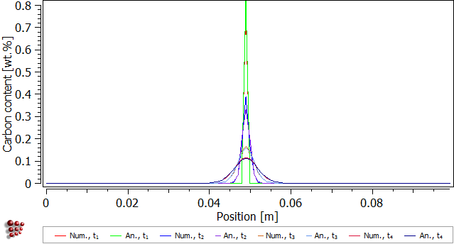
You will notice that, at first, the peak value of the analytical expression is much higher than the maximum value of 0.8 wt. % in the numerical simulation. The reason for this is that the analytical solution is based on the assumption that all the carbon is initially in an infinitesimally thin layer, whereas in the numerical solution, we have put the carbon into a cell of finite thickness. As the simulation proceeds, the two curves start to approach each other until they eventually almost exactly coincide. By default, the profile plot is set to show a 'stepped' profile in which the concentration is shown as discrete values corresponding to the single concentration value assigned to each cell. In the options window for this plot, select no under use steps to instead see a smooth curve that may enable easier comparison with the analytical curve.

When the simulation is finished, you can examine the profiles at different times by looking at Global > Buffers > Edit Buffer States. You can obtain a set of profiles as shown below by loading up selected buffer states and using ‘Duplicate and Lock all Series’ on the plot right-click menu.

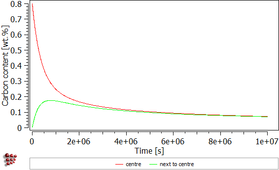
On the cell history plot, you should be able to see how the carbon concentration of the central cell decreases, while that of the adjacent cell decreases, until at longer exposure times, they converge.

Go to the MatCalc tutorial index.