Table of Contents
T10: T0-temperature in Fe-Cr-C
This tutorial was tested on
MatCalc version 6.04 rel 1.001
license: free
database: mc_fe.tdb
Complimentary files
Click here to view the script for this tutorial.
Click here for .xls or here for .txt table, respectively.
Contents:
- T0- temperature calculation
- Martensite / Bainite transformation
- Variation of T0- temperature with carbon and chromium content
- Import and display of experimental data into plots
The T0-temperature is defined as the temperature where two phases of identical chemical composition have the same molar Gibbs free energy. This temperature is an important quantity in the field of diffusionless phase transformations, i.e. the bainitic and martensitic transformation. In the present example, we will discuss some thermodynamic aspects of the austenite/martensite transformation and apply T0-temperature calculations to the evaluation of transformation temperatures.
Step 1: Define the thermodynamic system (see also Tutorial T2)
Create a new workspace file. From a suitable database (mc_fe.tdb) define the elements Fe, Cr and C as well as the phases BCC_A2 (ferrite) and FCC_A1 (austenite). Enter the system composition in weight percent with wp(C) = 0.1 and wp(Cr)=1.0. Set initial values with 'Calc' → 'Set start values' or Ctrl+Shift+F. Calculate an equilibrium at 800°C.
Step 2: Calculate the T<sub>0</sub>-temperature

Before evaluation of the T0-temperature, an equilibrium located in the one-phase region of the parent phase must be calculated in order to set the composition of one of the phases equal to the system composition. The parent phase is austenite so the solubility temperature of BCC_A2 will be evaluated with 'Calc' → 'Search phase boundary…' or Ctrl+Shift+T. Set 'Temperature' as type and 'BCC_A2' as target phase, then click on 'Go'. As a result, MatCalc displays in the 'console' window
Tsol 'BCC_A2': 857,21 C (1130,36 K) iter: 12, time used: 0,02 s
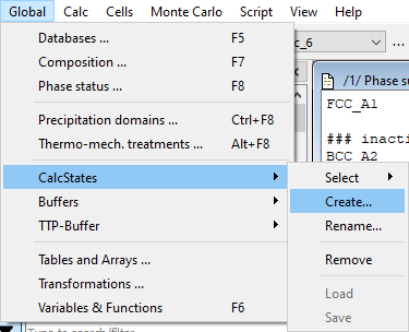
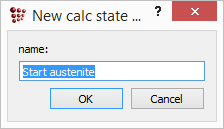
In the 'Phase summary' and 'Phase details' window, only the FCC_A1 phase is denoted as active (mole fracton = 1). We can now proceed with this initial condition. For convenience, store this (current) state in a calculation state with the name 'Start austenite' by selecting 'Global' → 'CalcStates' → 'Create…'.
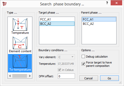
We can now evaluate the T0-temperature for austenite and ferrite with 'Calc' → 'Search phase boundary…' or Ctrl+Shift+T. The following, well-known, dialog box appears:
Select 'T0-temperature' in the type listbox, 'BCC_A2' as target phase and 'FCC_A1' as parent phase. The check box 'Force target to have parent composition' must be chosen, because the composition of BCC_A2 wil be adjusted according to the parent composition. The energy difference (DFM offset) can be left as default (zero). Press 'Go' to start the calculation. The result is shown below
T0(FCC_A1/BCC_A2):  791,461 C (1064,61 K)
iter: 2, time used: 0,00 s
- OK -
The phase details window shows:
#### /FCC_A1/ moles: 1, gm: -46908,9 (-46908,9)
Phasestatus: entered - active
FE +9,84677e-001  CR +1,06937e-002   C +4,62933e-003


### inactive ###

#### /BCC_A2/ moles: 0, gm: -46908,9 (-46908,9)
Phasestatus: entered - not active (dfm=2,4156e-009)
FE +9,84677e-001  CR +1,06937e-002   C +4,62933e-003
It is thus clear that, at the temperature of 791,461°C, FCC_A1 and BCC_A2 of the same composition have the same molar Gibbs free energy of gm = -46908.9 J/mole.
Step 3: Evaluate T<sub>0</sub>- temperature as a function of chromium content

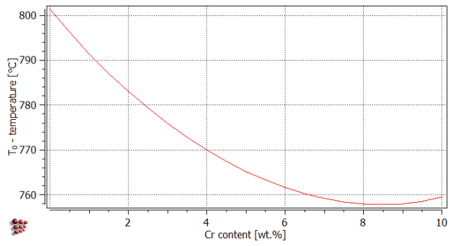
Let us now investigate how the T0- temperature for ferrite and austenite varies with the chromium content. From the menu select 'Calc' → 'Stepped calculation…'or press Ctrl+T. In the left listbox of the 'Step equilibrium …' window, select type 'T0 temperature'. Select 'FCC_A1' for the parent phase and 'BCC_A2' for the target phase. Don't forget to select chromium as the independent element. Enter the chromium range between '0' and '10' weight percent in steps of '0.5' and don't forget to mark the 'Force identical composition' box. The 'Step equilibrium …' window looks now as follows.
Press 'Go' to start the calculation. The result can be displayed in the well known 'XY-data' plot. Create the plot and drag and drop the T$c variable from the variables window into the plot. Edit the 'x-axis', 'y-axis' and 'legend' (see also Tutorial 4 or Tutorial 5) such that the result of the stepped T0- temperature calculation looks as follows.
Step 4: Evaluate T<sub>0</sub>-temperature as a function of carbon content

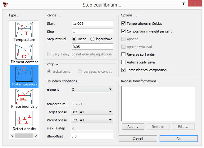
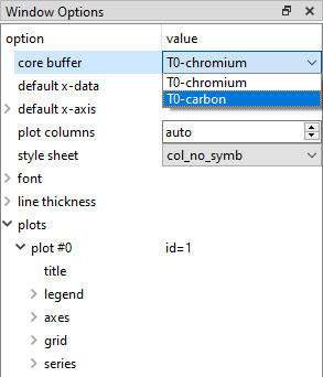
In the same way, similar to the evaluation of the dependence of the T0- temperature on the chromium content, it is possible to calculate the T0- temperature as a function of the carbon content. Therefore, rename the '_default_' buffer selecting 'Global' → 'Buffers' → 'Rename…' and give it the name 'T0-chromium'. Then create a new buffer ('Global' → 'Buffers' → 'Create…') with the name 'T0-carbon' and load the calculation state 'Start austenite' (make sure that the current buffer is the 'T0-carbon'). Analogously to the calculation before, carry out a stepped calculation. Press 'Calc' → 'Stepped calculation …' or press Ctrl+T, enter the following settings and press 'Go'.
There is no need to create a new plot in order to display the graph for the T0-temperature dependence for varying carbon content. The T0- temperature line in the figure can be simply changed by switching from 'T0-chromium' buffer to the 'T0-carbon' buffer in the options window.
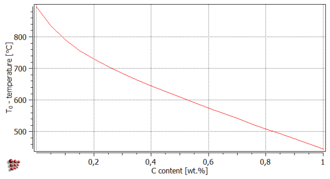
Afterwards, the x- and y-axes must be rescaled and in the case of the x-axis renamed. So the result looks as follows.
The strong dependence of the T0- temperature on the carbon content is evident. This is reflected in the strong influence of carbon on the martensite start temperature.
Step 5: Add some experimental data on martensite start temperatures
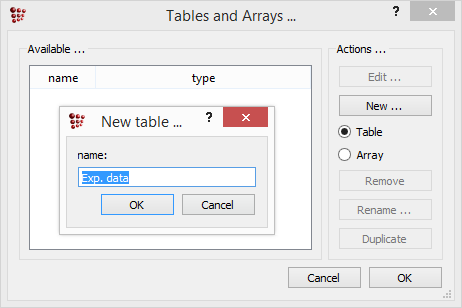
The experimental data, which will be added to the recent plot, are taken from ref. 1). Before doing so, we must create a new buffer. So, none of the former results will be lost. Name the new buffer as 'T0 with offset' (further calculations with various dfm-offsets will be done …) and create a table selecting 'Global' → 'Tables and Arrays'. Press 'New …' and call the table 'Exp. data'.
After selecting 'Edit …', enter the following measured martensite start temperatures into the table or copy them from a file (the file is here, or here (.txt)).
| Carbon content[wt%] | Martensite start temperature |
|---|---|
| 0 | 540 |
| 0.086 | 510 |
| 0.1936 | 475 |
| 0.2409 | 480 |
| 0.2495 | 470 |
| 0.2581 | 440 |
| 0.3011 | 430 |
| 0.3226 | 410 |
| 0.3871 | 410 |
| 0.3871 | 400 |
| 0.3871 | 395 |
| 0.4560 | 405 |
| 0.4947 | 355 |
| 0.5054 | 375 |
| 0.6022 | 330 |
| 0.6022 | 320 |
| 0.7097 | 280 |
| 0.7312 | 280 |
| 0.7743 | 265 |
| 0.8173 | 240 |
| 0.8603 | 225 |
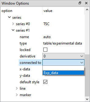
Press 'OK' twice and insert the experimental data into the plot as a new series (right-click in 'options' window and select 'New series' → 'table experimental data') and switch to 'Exp. data' in 'connected to' box (see also Tutorial 5).
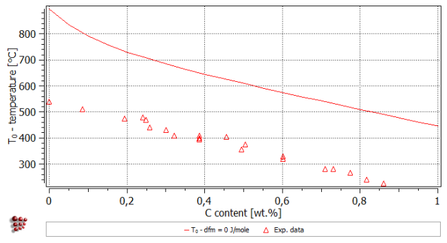
Edit the legend and the series names. The result looks as follows.
Apparently, the calculated T0- temperature does not fit the experimental data, however the curve runs parallel to it with the calculated temperatures being higher. The reason is that a certain amount of driving force is required to start the martensite transformation. This extra energy, or extra driving force, is of the order of 1.2 to 2.5 kJ/mol (depending on the composition of the alloy) and can be defined in the field dfm-offset. Default value for this parameter is zero.
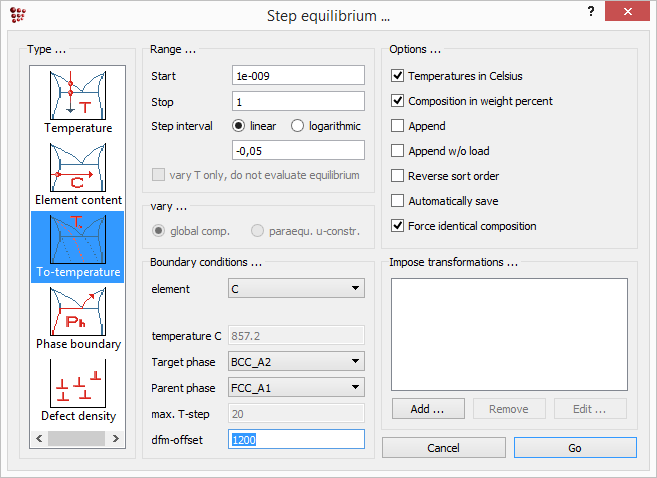
To evaluate how high this extra energy is as a function of carbon content, stepped calculations with different dfm-offsets can be performed. Carry out two simulations, one as a steped T0- temperature calculation with a dfm-offset of 1200 J/mole and one with 1700 J/mole. Before starting, lock the first series (T0- dfm=0 J/mole). So the first graph will be conserved for further comparison. Select 'Calc' → 'Stepped calculation …'and complete the dialog box as follows:
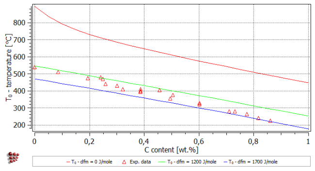
Change the plot buffer to 'T0 with offset' in the 'options' window. Drag and drop the 'T$c' variable again into the plot and rename the series to T0 - dfm=1200 J/mole. Lock the curve afterwards. Repeat these operations to obtain a curve for a dfm-offset of 1700 J/mole. The plot now looks like follows.
A dfm-offset in the range of 1200-1700 J/mole can be used to obtain reasonable agreement between the calculations and the experimental data.
Consecutive articles
The tutorial is continued in article T11 - Simulation of solidification of 0.7C 3Mn steel
Go to MatCalc tutorial index.
[1] Z. Jicheng and J. Zhanpeng, Acta met. mater. 38 (1990) 425-431.
