Table of Contents
Example H1: Heating a block of metal
Compatibility
MatCalc version: 5.44.0015
Database: none
Author: Manuel Oschgan
Created: 2008-2009
Revisions: 28.10.2011 (Update for 5.44, Georg Stechauner)
Objectives
The block (20 cm x 20 cm) is simulated as a two dimensional problem. This means that there is only one cell used for calculation in the third dimension. The dimensions are twice as big in reality as in the simulation, since only a fourth of the block needs to be simulated, because symmetric boundary conditions are used. The heating process is done in an oven, therefore the oven-temperature is a time-dependent. The heating process starts a bit higher than room temperature (300 K), takes approximately 20 minutes, and the block is heated up to 750 K. Convection heats the block, so that is the boundary condition used in MatCalc.
The questions that should be answered are:
- What is the temperature distribution in the block, after 20 minutes of heating?
- How fast does the temperature rise in dependence of the oven temperature?
A practical case could be that each cell of the block has to reach a required minimum temperature. This can help to decide if the heating time of 20 minutes is enough.
The step by step description is combined with MatCalc commands and the whole script is included below. For details, on how to enter commands or run a script, check the MatCalc Tutorials. This example uses only the simulation module and no databases are needed, because only temperature field simulation is used. However, currently not all functions of MatCalc are available if no database is loaded, so if some of these functions are needed, databases have to be loaded.
Important note
Related documents
None
Complementary files
Click here to view the script for this tutorial.
Main document
Setup system
USE_MODULE SIMULATION
NEW_WORKSPACE
At first, the simulation module is loaded and a new workspace is created.
NEW_GUI_WINDOW g5
SET_VARIABLE_VALUE paint_window_id active_frame_id
MOVE_GUI_WINDOW paint_window_id 0 100 600 750
The grid window of the type 'Paint grid:2D cells' is created that will show the temperature in grey scale. To be able to modify options of this window, the ID of the window is saved in the variable 'paint_window_id'. The last command sets the x/y position and width/heigth to a desired value.
SET_VARIABLE_VALUE gsize 10
SET_VARIABLE_VALUE hgsize (gsize+1)/2
The SET_VARIABLE_VALUE command, in MatCalc, sets an existent variable to a specified value or creates a new variable with that value if none exists yet. The first parameter is the variable name and the second parameter specifies which value is to be used. If this parameter is omitted, the user is prompted to enter a value. The variable gsize will be used, to determine how many cells exist in x and y direction. Since this is a two dimensional problem, there is only one cell in z direction. The variable hgsize is used later, to draw the plots of the center of the block.
SET_VARIABLE_VALUE min_trange 200
SET_VARIABLE_VALUE max_trange 1000
SET_VARIABLE_VALUE sim_time 1210
To specify the time scale of the plots, the variables 'min_trange' and 'max_trange' are used. For setting the simulation time, the variable sim_time will be used later.
CREATE_SIMULATION_GRID gsize gsize 1
SET_GRID_COORDINATES 0.2 0.2 1
The simulation grid is created with gsize cells in the x-direction and y-direction, respectively. The z-direction has only one cell. With the grid coordinates, the dimensions of the whole grid in each direction are defined. In this example the grid is 20 cm in x/ y direction and 4 cm in z direction.
SET_VARIABLE_VALUE gsize gsize-1
SET_VARIABLE_VALUE hgsize hgsize-1
The variables gsize and hgsize are decremented by one, because they are now used, to access the grid that has a starting index of zero.
CREATE_MATERIAL ferrite
SET_MATERIAL_PROPERTY ferrite T D 7890	 $ density
SET_MATERIAL_PROPERTY ferrite T C 500	 $ heat capacity
SET_MATERIAL_PROPERTY ferrite T N 50	 $ thermal conductivity
SET_MATERIAL_PROPERTY ferrite T E 10000	 $ thermal grain boundary diffusion enhancement
A new material named 'ferrite' is created, in order to simulate the thermal properties correctly. Therefore the parameters density, heat capacity, thermal conductivity and the thermal grain boundary diffusion enhancement are set to the desired values. The correct units for the parameters can be checked by entering the commands manually, without the value.
Setup simulation and output parameters
SET_SIMULATION_PARAMETER N N
Since in the whole example kelvin is used as temperature unit, the simulation parameter 'Temp in °C' is set to 'No'.
SET_GUI_WINDOW_PROPERTY paint_window_id i Z 100 $ zoom 100%
SET_GUI_WINDOW_PROPERTY paint_window_id i W V $ display cell variable
SET_GUI_WINDOW_PROPERTY paint_window_id i V _ct $ set which variable
SET_GUI_WINDOW_PROPERTY paint_window_id I R min_trange..max_trange
In order to customize the grid window, the zoom is set to 100%, the display is set to show the cell variable (possible would be also show the selection, boundary conditions and other options) and the cell variable is set to '_ct' (cell temperature). Please note that in previous versions of MatCalc this variable was defined without the underscore. The value range of the cell variable is set to min_trange..max_trange (means the grid will show temperatures between min_trange and max_trange kelvin as defined by the variables).
NEW_GUI_WINDOW g1
SET_VARIABLE_VALUE profile_window_id active_frame_id	$ remember window id
SET_VARIABLE_VALUE profile_plot_id last_plot_id	 $ remember plotid
SET_PLOT_OPTION profile_plot_id S N S _ct
CREATE_NEW_PLOT 1 profile_window_id
SET_VARIABLE_VALUE profile_plot2_id last_plot_id
SET_PLOT_OPTION profile_plot2_id S N S _ct_dot
A new 'Plot-grid: 1D profile' window is created. The window ID and the plot ID of the first plot, which is automatically created, are saved. The first plot is configured to show the variable _ct (cell temperature) and another plot is created, with the plot ID also being stored. To show the time change of the temperature in the second plot, the variable _ct_dot is used. The x-axis in such profile plots shows the position in the grid as default setting. The variable can be customized, though. Please again note that in contrast to former tutorials, the cell variables, now, have to be prefixed by an underscore.
SET_GUI_WINDOW_PROPERTY profile_window_id I T 0.hgsize.0
SET_GUI_WINDOW_PROPERTY profile_window_id I o gsize.hgsize.0
MOVE_GUI_WINDOW profile_window_id 530 100 460 800
In order to define which content is shown on the x axis, the first two commands define the start and end coordinates of the cells, which are displayed in the plot. Each directions cell numbering starts at zero. 't 0.hgsize.0' defines that the profile plots x-axis starts with values of the cell 0.hgsize.0 (x.y.z). 'o gsize.hgsize.0' means that the last cell on the x-axis will be the gsize.hgsize.0 cell. After that, the window is moved to a proper position and sized accordingly.
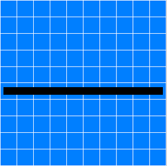
Fig. 1: Grid window showing a grid of 10×10 cells. The black bar covers the cells being displayed by the profile plot.
NEW_GUI_WINDOW g2
SET_VARIABLE_VALUE history_window_id active_frame_id	$ remember window id
SET_VARIABLE_VALUE history_plot_id last_plot_id	 $ remember plotid
SET_PLOT_OPTION history_plot_id A X 1 T time - s
SET_PLOT_OPTION history_plot_id A Y 1 T temperature - K
SET_PLOT_OPTION history_plot_id A X 1 S 0..sim_time
SET_PLOT_OPTION history_plot_id A Y 1 S min_trange..max_trange
SET_VARIABLE_VALUE fact gsize/4
SET_PLOT_OPTION history_plot_id S N S _ct{0.fact-1}
SET_PLOT_OPTION history_plot_id S N S _ct{0.fact*4-2}
SET_PLOT_OPTION history_plot_id S N S _ct{fact*2.fact-1}
SET_PLOT_OPTION history_plot_id S N S _ct{fact*2.fact*4-2}
SET_PLOT_OPTION history_plot_id S N S _ct{fact*4-1.fact-1}
SET_PLOT_OPTION history_plot_id S N S _ct{fact*4-1.fact*4-2}
A new gui window, which will be used to display the time evolution of some cells, is created. After storing its window id and plot id, the captions of the axes are set and the ranges are corrected to fit to the example. Six new series are attached to the history plot, each of them showing the cell temperature of a specific cell. The cell temperature (variable _ct) is indexed using the format x.y in the braces. To calculate which cells should be shown on the plot, the variable “fact” is dependent on the grid size.
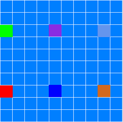
Fig. 2: The colored cells in the grid window are drawn using the same color in the history plot.
SET_CELL_PROPERTY A V T 300 $ set selected cells to 300 K
SET_CELL_PROPERTY A M ferrite $ attach material to those cells
Using the SET_CELL_PROPERTY command, all cells are set to a temperature of 300 K (parameter A stands for all cells) and the ferrite material is attached, also.
SET_SIMULATION_PARAMETER e sim_time $ simulation end time
SET_SIMULATION_PARAMETER u 10 $ update every
SET_SIMULATION_PARAMETER T F
After the simulation end time is set (sim_time seconds), the plots update interval is changed to ten seconds. Also, the type of calculation has to be chosen, before starting simulation. 'T F' means temperature → temperature field simulation.
SET_PLOT_OPTION profile_plot_id A Y 1 S min_trange..max_trange
SET_PLOT_OPTION profile_plot2_id A Y 1 S -1..5
SET_PLOT_OPTION profile_plot_id l N
SET_PLOT_OPTION profile_plot2_id l N
SET_PLOT_OPTION profile_plot_id A Y 1 T T - K
SET_PLOT_OPTION profile_plot2_id A Y 1 T dT/dt - K/s
SET_PLOT_OPTION profile_plot_id A X 1 T distance - m
SET_PLOT_OPTION profile_plot2_id A X 1 T distance - m
To get nice plots some options are configured. The ranges for both y-axes are set accordingly (min_trange..max_trange K, 0..5 K/s), a legend is disabled for each plot and the axe titles are also changed.
CREATE_BOUNDARY_CONDITION T C 3000
SET_CELL_PROPERTY 0.gsize..gsize.gsize B A 0 U
SET_CELL_PROPERTY 0.gsize..c0.0 B A 0 L
Now, the boundary condition is created. It is a convection boundary condition of 3000 W/(m²K). To assign the boundary condition (with index 0 because only one exists) to the correct cells, their cell properties are set accordingly and the BC is attached. As you can see, the variable gsize is used to determine, which cell range the boundary condition has to be attached. The second line attaches the condition to the upper border of the block and the third line to the left border. The parameter U(up) and L(left) define which side of a cell is exposed to convection. In order to simulate only 1/4 of the block, the default geometric boundary condition for the sides, with no boundary conditions attached, is symmetric.
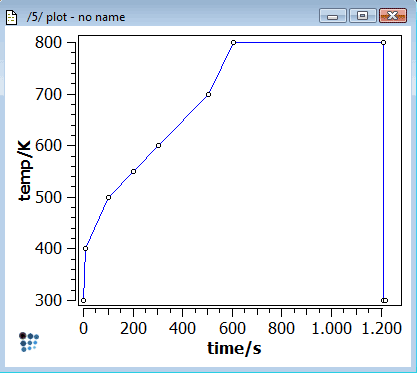
CREATE_GLOBAL_TABLE oventemp
ADD_TABLE_ENTRY oventemp 0 300
ADD_TABLE_ENTRY oventemp 10 400
ADD_TABLE_ENTRY oventemp 100 500 $ 1,6 min
ADD_TABLE_ENTRY oventemp 200 550 $ 3 min
ADD_TABLE_ENTRY oventemp 300 600 $ 5 min
ADD_TABLE_ENTRY oventemp 500 700 $ 8,3 min
ADD_TABLE_ENTRY oventemp 600 800 $ 10 min
ADD_TABLE_ENTRY oventemp 1200 800 $ 20 min
ADD_TABLE_ENTRY oventemp 1202 300 $ 20 min
ADD_TABLE_ENTRY oventemp 1210 300 $ 20 min
To simulate the oven, with changing temperature, a table is created that holds all temperature values. 'oventemp' is the table name. The ADD_TABLE_ENTRY command inserts an enrty that consists of two parameters, a key and a value. Every value in the table can be accessed by its key. If the key does not exist the value of the missing key is linear interpolated through the neighbor entries. That means in our case, the key will be used as time in seconds and the value will be the oven temperature. If the temperature at a given time is needed, the table returns the appropriate value by accessing 'oventemp(mtime)'. Here mtime is a variable that has been set by the user, before. A plot of the table is shown below.
Set boundary condition
SET_DEFAULT_BOUNDARY_COND T oventemp(_ctime)
The ambience temperature, at a given time, is determined by the values in the table. This is accomplished by setting the default boundary condition for the ambience temperature. A boundary condition parameter can be a function that is evaluated during simulation time. In this case, the function only consists of a table with the parameter '_ctime' in the brackets. It is the variable cell time that holds the current simulation time and is used as index for the table access.
Start Simulation
All cells are now blue, which stands for a temperature of 300 K in this example. Now, the simulation can either be started by using the main menu command or via the shortcut Ctrl + J. The evolution of the grid window is shown below:

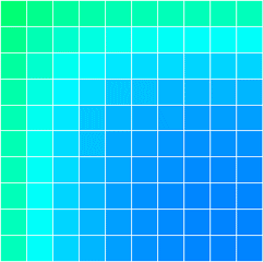
Fig. 4: Left: 100 seconds; border temperature of 400 K. Right: 203 seconds; border temperature of 460 K; spreading of heat to the core.
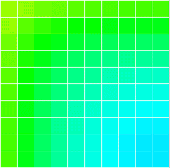

Fig. 5: Left: 600 seconds; outside: 740 K - 550 K; core: 380 K. Right: 1210 seconds; border temperature of 770 K; core: 590 K.
The block begins to heat from the top and left sides since the convection boundary condition is attached there. Only a quarter of the block is simulated; the other two sides are symmetric and heat slower (core heats slower). At first only the boundaries are heated significantly. After 300 seconds also the innermost of the block begins to heat.
The evolution of the plot windows looks as follows:
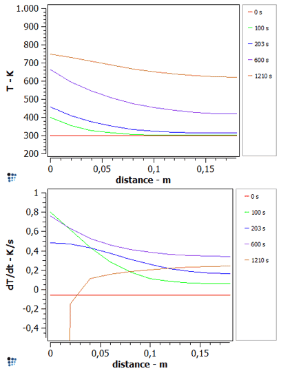
Fig. 6: Every line shows the temperature distribution of the cells marked in figure 1 at a specific time.
As shown in figure 6 the cells on the left side start to heat at first and also the gradient is the highest there at the beginning (green curves). After some time the temperature change increases to the core and has to decrease at the border because the ambience temperature stays constant after 600 seconds. At 1200 seconds, the temperature has reached its maximum in all cells, and decreases a bit on the outside, because the block is taken out of the oven (300 K ambience temperature). The decrease after 1200 seconds is shown in the dT/dt plot by the brown series. The specific curvatures of the different dT/dt series are dependent on the oven characteristic.
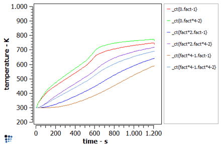
Fig. 7: Time evolution of the cells marked in figure 2.
In figure 7 the border cells (green and red) are more curved at 600 seconds because at this point the oven temperature stays constant. The change at the inner cells is more smooth, the oven temperature does not affect them as strong.
Consecutive articles
None
