MatCalc version: 5.52.0038
Database: mc_fe.tdb (newest version!), mc_sample_fe.ddb
Author: Georg Stechauner
Created: 2013-08-28
Revisions:

This final part shows the calculation of the TTP curve for Cu precipitates in the binary Fe-Cu system. We will consider all the information which was worked out in the prior parts. Therefore, the settings which are used here, will not be discussed.

There are basically two ways on how to create the TTP curves which will be shown: (a) setthe system up according to part 2, and use the “Calc → TTP diagram” function from the menu. Use the correct temperature borders and MatCalc will perform the simulation. (b) The second approach needs a little scripting, or just use the supported one: the main difference is the fast cooling prior to isothermal holding, which leads to creation of thermal vacancies. It will be shown however, that the influence of them is neglectable.

It is up to you to decide, whether to use the script or to simple use the GUI function.

Note: This is an advanced example and will not cover basics like “How to create a plot”, etc… . Please consider earlier P-examples for instructional purpose.

• P80-1 - Models and parameters for Fe-Cu simulation
• P80-2 - Precipitation of Cu in Fe-Cu
• M. Perez, F. Perrard, V. Massardier, X. Kleber, V. Schmitt, A. Deschamps, Low Temperature Solubility Limit of Copper in Iron, Materials Science Forum 500-501 (2005) 631-638.

Click here to view the script for this example.

Set up the thermodynamics, precipitates, domains, … according to part 2. Or simply load your prior workspace

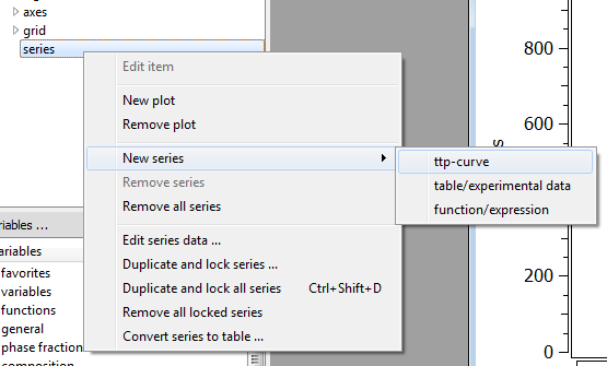
Create a new P6 - TTP plot. Click into the plot, and navigate to the 'options…' window on the left side, and right click on 'series'. Select 'New Series –>' and 'ttp-curve'.

To display the sum-curve of all precipitates and to include the transformation, we need to choose 'use_x_data_string' as data. Otherwise we could only choose from one of the three present phases. Enter the sum as 'f$cu_bcc_1_p0+f$cu_bcc_2_p0+f$cu_fcc_p0' in the x-data field. Enter '0.10' for y-data, to display the 10% phase fraction line. In the general plot options, select 'relative' at 'refer to f'. This will consider the maximum phase fraction of each temperature as 100% and refer the 10 line to it.

When using the GUI, simply select the according menu item in Calc → TTP diagram, or use the short-cut Ctrl-Alt-K. We use the temperature borders of 400 and 700°C.

Attention: The simulation gets unstable at high temperatures which will lead to oscillations an numerical problems. MatCalc will try to keep on simulating, which leads to very long simulation times. To solve this, only calculate up to 650°C or stop the simulation manually once the problem occurs.

The GUI version also needs regular input if you want to proceed with the next temperature.

Therefore, it is suggested to use the provided script with the TTP-loop.

ATTENTION: Using the GUI can result in errors due to wrong phase-fraction calculation. Be aware of that when checking your results!

The biggest amount of the script is similar to part 2 of this example. The most important piece of code, is the TTP-calculating-loop at the very end.

for (j;400..850;25)
  $ Create buffer states for each temperature and name them 
  format-variable-string buffer_name "buffer_%d" j 
  create-calc-buffer #buffer_name
  set-gui-window-property buffer_window_id b #buffer_name

  set_simulation_parameter t c 850 -100 10 
  set_simulation_parameter m j
  set_simulation_parameter s r
  set-precipitation-parameter cu_bcc_1_p0 n s n  $ nucleation sites are none
  start-precipitate-simulation
  create-calc-state cool
  
  set_simulation_parameter s l cool
  SET_SIMULATION_PARAMETER T i j                 $ (I)sothermal at temperature "j"
  set_simulation_parameter e 1e11                $ End time 
  set-precipitation-parameter cu_bcc_1_p0 n s b  $ nucleation sites are bulk
  $calculate-equilibrium j
  start-precipitate-simulation
  $edit_ht_segment ht 1 1 j 10 
  
  append-ttp-buffer
  
endfor

This portion of code first creates a buffer, corresponding to the actual simulation temperature. After that, it quenches quickly to isothermal holding temperature, to consider the effect of quenched in vacancies. The last part actually starts the simulation and appends the results from the buffer to the ttp-buffer.

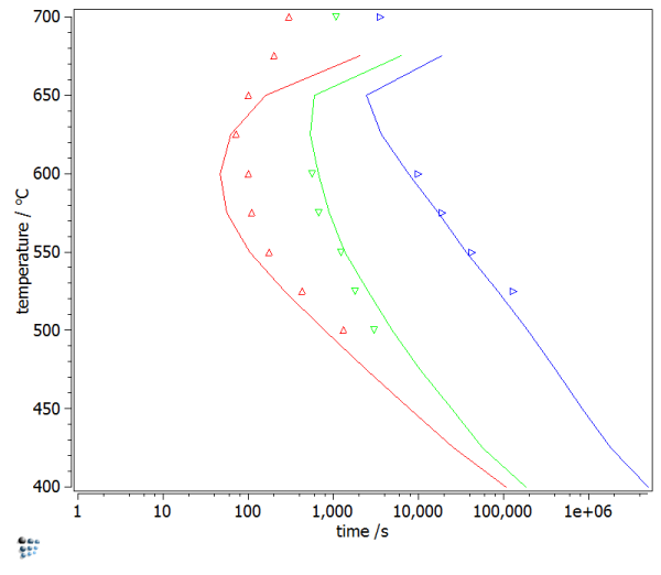
The resulting TTP-Plot should look similar to this one. Errors and numerical problems can occur above the 650°C point with the automatic plot.

None