Table of Contents
Example P12: NbC precipitation in steel
Compatibility
MatCalc version: 5.60
Database: mc_fe.tdb, mc_x_FeAlCCrMnNSiV.tdb, mc_sample_fe.ddb
Author: Walter Mayer
Created: 2012-06-07
Revisions: Heinrich Buken 2014-03-18
Objectives
This example deals with the precipitation of NbC in a low alloyed steel. The location of nucleation is considered in dislocations as well as on grain- boundaries.
Main document
Setup thermodynamics
Set up the thermodynamics by either loading the mc_fe database, or the corresponding example database mc_x_FeAlCCrMnNSiV.
Select the following phases, elements and enter the chemical composition in wt-%:
| Elements | Chemical composition | Phases |
|---|---|---|
| Al | 0.001 | BCC_A2 |
| C | 0.009 | FCC_A1 |
| Mn | 0.001 | |
| N | 0.001 | |
| Nb | 0.105 | |
| Ti | 1e-08 |
Set Fe to reference element.
Conclude the thermodynamic setup by loading the diffusion database for Fe.
Precipitation domain and precipitates
Go to the phase status dialog mark FCC_A1 and press create. Choose composition set type the following: :NB%:C,VA%: and name the phase NbC. Now mark the new NbC phase push the create button mark the precipitate (_Pnn) and press OK. Repeat the last step (select NbC and choose precipitate) and you will find three new phases in the list: NbC, NbC_P0, and NbC_P1.
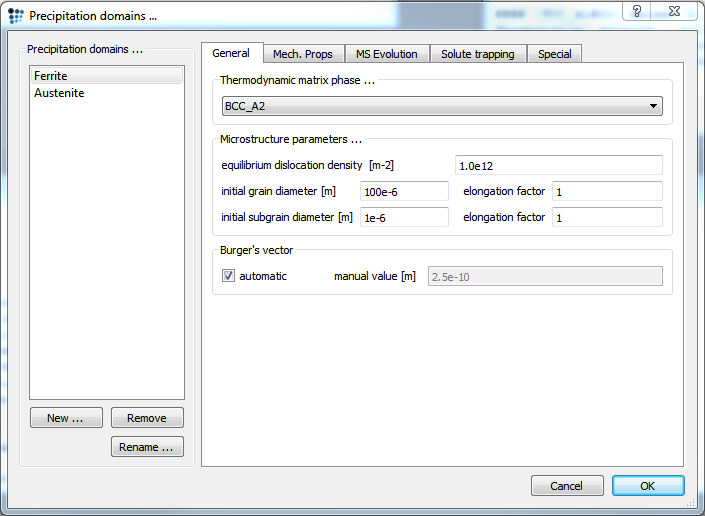
Next we enter the data for the precipitation domain. To do so, open the precipitation domain dialog and create a new domain. Select fcc_a1 as its matrix phase and name it “Austenite”. Build a second precipitation domain name it Ferrite and choose bcc_a2 as its matrix phase. Leave the domain settings as they are.

Follow by adjusting the precipitates. Bring up the phase status dialog window and select the NbC_Px phases.
| Precipitate | Tab | Option | Value |
|---|---|---|---|
| NbC_p0 | Precipitate | #size classes | 25 (Initialize!) |
| NbC_p0 | Nucleation sites | grain boundary |
| Precipitate | Tab | Option | Value |
|---|---|---|---|
| NbC_p1 | Precipitate | #size classes | 25 (Initialize!) |
| NbC_p1 | Nucleation sites | dislocations |
Start precipitation simulation
To ensure correct thermodynamic values and no driving force errors (DFM-errors), set automatic start values and calculate an equilibrium at 1250C.
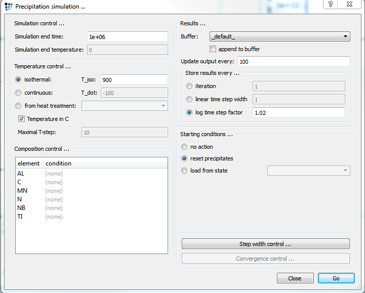
Open “precipitation kinetics…” and calculate the evolution of the NbC precipitations at 900°C.
Press “Go” to start the heat treatment.
Plotting the results
Create a new X-Y-Plot (p1) and add two new plots. Set a default x-axis to logarithmic with a scaling from 1e-6.. and label the axis time / s.
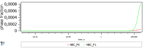
- Plot the phase fractions of the precipitates in the first figure (
f_prec$…) and the corresponding experimental data from the table. - Plot the mean radius of the precipitates in the second figure (
r_mean$…). Add a scaling factor of 1e9 to display the size in nm. - Plot the number density of the precipitates in the third figure (
num_part$…).
Label the y-axes accordingly.
A quicker way of depicting the demanded diagramms is to create a user defined window (select “03_kinetics_4frames_T_f_n_r_linX” and remove the temperature-plot).


