Table of Contents
Example P10: AlN precipitation in steel, part 2: AlN precipitation in ferrite
Compatibility
MatCalc version: 5.44.1002
Database: mc_fe.tdb, mc_x_FeAlCCrMnNSiV.tdb, mc_sample_fe.ddb
Author: Georg Stechauner
Created: 2012-01-18
Revisions:
Objectives
Before starting with this example, make sure that you have already worked through P10-1 as they are very similar.
Whilst example P10-1 covered the precipitation of AlN in austenite, this example will treat the precipitation in ferrite. Thus, the procedure of setting up the system is very similar. However, the script is more complex, as it involves user interaction. The setup of the if-conditions will be covered during this example.
The experimental data is taken from Massardier et al. (see cited literature). The paper is about the precipitation of nitrides in a low alloy aluminum killed steel. The free nitrogen contents were measured by utilizing thermoelectric power (TEP) measurements.
Related documents
- P10-1 - AlN precipitation in austenite
- P10-2 - AlN precipitation in ferrite
- V. Massardier, V. Guetaz, J. Merlin, M. Soler, Kinetic and microstructural study of aluminium nitride precipitation in a low carbon aluminium-killed steel, Materials Science and Engineering A355 (2003) 299-310
Complementary files
Click here to view the script for this tutorial.
Main document
Setup thermodynamics
Set up the thermodynamics by either loading the mc_fe database, or the corresponding example database mc_x_FeAlCCrMnNSiV.
Select the following phases, elements and enter the chemical composition in wt-%:
| Elements | Chemical composition | Phases |
|---|---|---|
| Al | 0.058 | AlN |
| C | 0.025 | BCC_A2 |
| Cr | 0.039 | |
| Mn | 0.2 | |
| N | 0.005 |
Set Fe to reference element.
Conclude the thermodynamic setup by loading the diffusion database for Fe.
Experimental data
To be able to plot all three temperatures, which are available to select from in the script, you need to enter them into your workspace. If you are satisfied with only seeing one curve, and check the other results by running the script, feel free to do so.
Create three tables and enter the following values:
| Exp_T600 | Exp_T650 | Exp_T700 | |||
|---|---|---|---|---|---|
| x-Value: time / s | y-value: phase fraction | x-Value: time / s | y-value: phase fraction | x-Value: time / s | y-value: phase fraction |
| 300 | 2.667e-5 | 120 | 3.333e-5 | 60 | 8e-5 |
| 600 | 3.333e-5 | 240 | 5.333e-5 | 120 | 0.0001067 |
| 1200 | 5.333e-5 | 480 | 8e-5 | 180 | 0.0001733 |
| 2400 | 0.0001 | 780 | 0.0001466 | 240 | 0.00024 |
| 3600 | 0.0001333 | 1200 | 0.00016 | 480 | 0.00032 |
| 5400 | 0.00017333 | 1800 | 0.00023 | 900 | 0.0003466 |
| 12000 | 0.0003066 | 3600 | 0.0003666 | 1800 | 0.0004133 |
| 24000 | 0.0003667 | 6600 | 0.0004 | 4200 | 0.0004 |
| 54000 | 0.0004133 | 13800 | 0.0004 | 6600 | 0.0004133 |
| 78000 | 0.0003866 | — | — | 13800 | 0.0004133 |
| — | — | — | — | 30000 | 0.0004133 |
Precipitation domain and precipitates
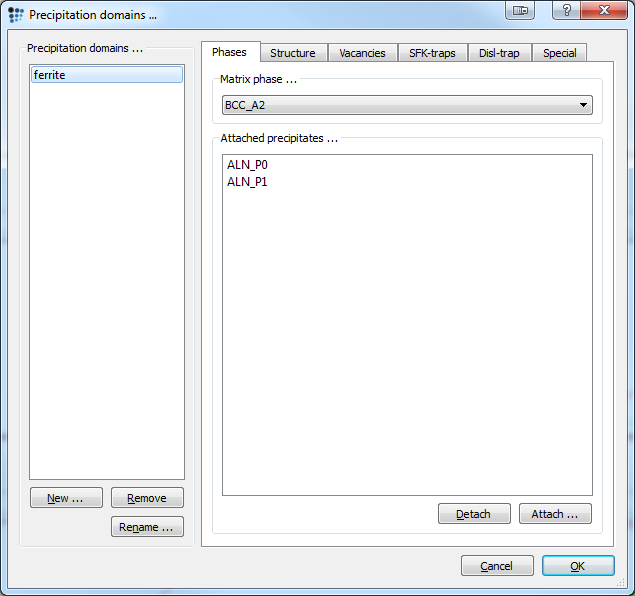
Next we enter the data for the precipitation domain. To do so, open the precipitation domain dialog and create a new domain. Select bcc_a2 as its matrix phase. Enter the following data in the corresponding tabs:
| Tab | Option | Value |
|---|---|---|
| Structure | Grain diameter | 7.5e-6 |
| Dislocation density | 1e12 | |
| Special | Young's modulus | (193000-73.333*T$C)*1e6 |
| Diffusion ratio grain boundary and bulk (substitutional) | (10^(12-0,01*T$C)) | |
| Diffusion ratio grain boundary and bulk (interstitional) | (10^(12-0,01*T$C)) | |
| Diffusion ratio dislocation and bulk (substitutional) | (10^(8-0,005*T$C)) | |
| Diffusion ratio dislocation and bulk (interstitional) | (10^(8-0,005*T$C)) |
Follow by setting up the precipitates. Bring up the phase status dialog window and select the AlN phase. Click 'Create new phase' and select 'precipitate'. Repeat this step to for a second population of AlN precipitates. Now begin with entering the parameters for AlN_p0 and then for AlN_p1:
| Precipitate | Tab | Option | Value |
|---|---|---|---|
| AlN_p0 | Precipitate | #size classes | 50 (Initialize!) |
| AlN_p0 | Attached to pd | ferrite | |
| AlN_p0 | Nucleation | Restrict nucleation to prec domain | ✔, select ferrite |
| AlN_p0 | Nucleation sites | grain boundary | |
| AlN_p0 | Structure | ignore for prec. strengthening | ✔ |
| Precipitate | Tab | Option | Value |
|---|---|---|---|
| AlN_p1 | Precipitate | #size classes | 50 (Initialize!) |
| AlN_p1 | Attached to pd | ferrite | |
| AlN_p1 | Nucleation | Restrict nucleation to prec domain | ✔, select ferrite |
| AlN_p1 | Nucleation sites | dislocations | |
| AlN_p1 | account for coherent misfit stress | ✔ | |
| AlN_p1 | Structure | volumetric misfit | No flag, enter 0.27 |
Understanding the script
As mentioned before, the script allows the user to choose one of three temperatures. To do so, two parts of the script are of interest:
set-variable-value sim_temp 1                         $ default value for calc variant

send-console-string
send-console-string Possible isothermal simulation temperature
send-console-string   1 ... T=600°C
send-console-string   2 ... T=650°C
send-console-string   3 ... T=700°C
input-variable-value sim_temp "Please select simulation temperature (1-3): "
The first line of the code sets a default value for the sim_temp variable. This is done to initialize the variable and to have value, if the user decides to simply press enter without entering a value.
The five lines send-console-string simply send the text behind the command to the console, so the user can read it. The last line input-variable-value is the line, where the user can choose between one of the three temperatures. The variable sim_temp will be set accordingly.
The second part of the temperature selection consists of some if-conditions:
if (sim_temp==1)
   set-variable-value temp 600                         $ value for isothermal simulation temp.
   set-variable-string exp exp_massardier_T600         $ exp. results for T=600°C
elseif (sim_temp==2)
   set-variable-value temp 650                         $ value for isothermal simulation temp.
   set-variable-string exp exp_massardier_T650         $ exp. results for T=650°C
elseif (sim_temp==3)
   set-variable-value temp 700                         $ value for isothermal simulation temp.
   set-variable-string exp exp_massardier_T700         $ exp. results for T=700°C
else
   send-dialog-string Invalid selection for simulation temperature. Select 1, 2 or 3.
   send-dialog-string Script is interrupted.
   stop-run-script  $ stop script
endif
The command if checks a condition in a boolean way: either the condition is TRUE, then the commands after the if will be performed, or the condition is FALSE, the the commands won't be executed and the script will jump to the next command, outside of the if.
The next command is an elseif, which can only follow an if. Should the first condition return FALSE, then this condition is checked. Is the return value again FALSE, the next command in line gets checked up to the point, were a simple else is found. The else command is performed and the endif closes the segment of the if-condition again.
Should the return of an if-condition be TRUE then the commands performed in this case are:
set-variable-value temp 600                         $ value for isothermal simulation temp.
set-variable-string exp exp_massardier_T600         $ exp. results for T=600°C
The first command sets the variable temp to 600, which will be the temperature for isothermal simulation later on. The second command saves the table, in this case 'exp_massardier_T600', to the variable-string exp. This makes the process of adding the correct experimental data to the plots later on easier.
Start precipitation simulation
To ensure correct thermodynamic values and no driving force errors (DFM-errors), set automatic start values and calculate an equilibrium at 1250C.
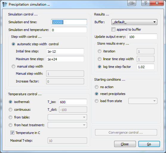
Open the precipitation simulation dialog, and enter the values as below. Vary the isothermal temperatures to simulate precipitation behaviour at other temperatures.
Note: The variable 'temp', which was set in the script above, is used here as the temperature value.
Plotting the results
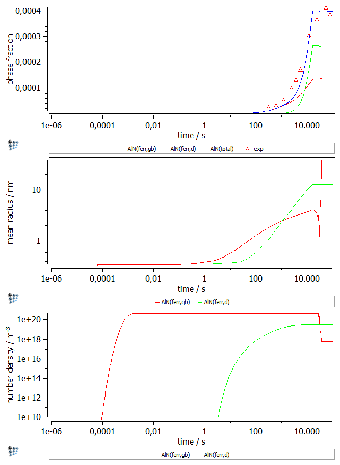
Create a new X-Y-Plot (p1) and add two new plots. Set a default x-axis to logarithmic with a scaling from 1e-6.. and label the axis time / s.
- Plot the phase fractions of the precipitates in the first figure (
f_prec$…) and the experimental data from the table. At a first glance it seems as if the calculated vales do not fit the experimental data. This is because the experimental data does not differentiate between the nucleation sites of the precipitates, whereas MatCalc does. Therefore, open the 'Functions & Variables' dialog window, an select the 'Functions' tab. Create a new function there and call itf_prec$AlN_totaland setf_prec$AlN_p0+f_prec$AlN_p1as its value. Now you can plot the total amount of precipitates. - Plot the mean radius of the precipitates in the second figure (
r_mean$…). - Plot the number density of the precipitates in the third figure (
num_part$…).
Label the y-axes accordingly.
The result for 600C is shown below:
Consecutive articles
none


