Table of Contents
Example P10: AlN precipitation in steel, part 1: AlN precipitation in austenite
Compatibility
MatCalc version: 5.44.1002
Database: mc_fe.tdb, mc_x_FeAlCCrMnNSiV.tdb, mc_sample_fe.ddb
Author: Georg Stechauner
Created: 2012-01-16
Revisions:
Objectives
This example is based on the paper of Leslie et. al. (1954) who have investigated the solution temperature of nitrogen and aluminum in aluminum killed steels. It is a goal to reproduce and simulate the measured data as good as possible. Therefore, many material and precipitation domain parameters will be entered. By measuring the nitrogen and aluminum contents, it was further possible to determine the concentration of AlN.
Related documents
- P10-1 - AlN precipitation in austenite
- P10-2 - AlN precipitation in ferrite
- Leslie et al., Solution and precipitation of aluminum nitride in relation to the structure of low carbon steels, Trans. ASM 46 (1954) 1470-1499
Complementary files
Click here to view the script for this tutorial.
Main document
Setup thermodynamics
Set up the thermodynamics by either loading the mc_fe database, or the corresponding example database mc_x_FeAlCCrMnNSiV.
Select the following phases, elements and enter the chemical composition in wt-%:
| Elements | Chemical composition | Phases |
|---|---|---|
| Al | 0.079 | AlN |
| C | 0.043 | FCC_A1 |
| Mn | 0.35 | |
| N | 0.0072 |
Set Fe to reference element.
Conclude the thermodynamic setup by loading the diffusion database for Fe.
Experimental data
A figure showing nitrogen content in matrix over time can be found in the cited literature. It is important to mention, that the researchers measured the nitrogen in wt-%, whereas MatCalc plots diagrams in mole fractions. Therefore the data gathered from the paper has to be converted by using the following formula 1):
\[AlN[mol\%] = \frac{m_{Fe}}{m_{N}} * x_{stoch} * N[wt\%]\]
where mFe/mN represents the difference in atomic weight (which is about 4) and xstoch takes the stoichiometric compound into account. The stoichiometric factor has a value of 2, as a measured value of AlN of one mole, consists of 50% Al and 50% N. Therefore one mole of nitrogen, can build two moles of AlN (assuming that Al is not the limiting partner). Thus a factor of 8 (4 * 2) must be considered when comparing the phase fraction of AlN in mol% to the measured amount of N in wt%.
Create a new table and enter the following values:
| x-Value: time / s | y-value: phase fraction |
|---|---|
| 120 | 9.6e-5 |
| 120 | 7.3e-5 |
| 600 | 0.000184 |
| 600 | 0.000168 |
| 6000 | 0.00037 |
| 6000 | 0.0004617 |
Precipitation domain and precipitates
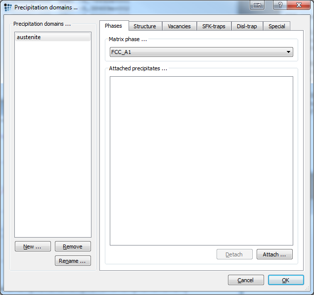
Next we enter the data for the precipitation domain. To do so, open the precipitation domain dialog and create a new domain. Select fcc_a1 as its matrix phase. Enter the following data in the corresponding tabs:
| Tab | Option | Value |
|---|---|---|
| Structure | Grain diameter | 50e-6 |
| Dislocation density | 1e11 | |
| Special | Young's modulus | (210000-75*T$C)*1e6 |
| Diffusion ratio grain boundary and bulk (substitutional) | (10^(11-0,005*T$C)) | |
| Diffusion ratio grain boundary and bulk (interstitional) | (10^(11-0,005*T$C)) | |
| Diffusion ratio dislocation and bulk (substitutional) | (10^(7-0,0025*T$C)) | |
| Diffusion ratio dislocation and bulk (interstitional) | (10^(7-0,0025*T$C)) |
Follow by setting up the precipitates. Bring up the phase status dialog window and select the AlN phase. Click 'Create new phase' and select 'precipitate'. Repeat this step to for a second population of AlN precipitates. Now begin with entering the parameters for AlN_p0 and then for AlN_p1:
| Precipitate | Tab | Option | Value |
|---|---|---|---|
| AlN_p0 | Precipitate | #size classes | 50 (Initialize!) |
| AlN_p0 | Attached to pd | austenite | |
| AlN_p0 | Nucleation | Restrict nucleation to prec domain | ✔, select austenite |
| AlN_p0 | Nucleation sites | grain boundary | |
| AlN_p0 | Structure | ignore for prec. strengthening | ✔ |
| Precipitate | Tab | Option | Value |
|---|---|---|---|
| AlN_p1 | Precipitate | #size classes | 50 (Initialize!) |
| AlN_p1 | Attached to pd | austenite | |
| AlN_p1 | Nucleation | Restrict nucleation to prec domain | ✔, select austenite |
| AlN_p1 | Nucleation sites | dislocations | |
| AlN_p1 | account for coherent misfit stress | ✔ | |
| AlN_p1 | Structure | volumetric misfit | No flag, enter 0.27 |
Start precipitation simulation
To ensure correct thermodynamic values and no driving force errors (DFM-errors), set automatic start values and calculate an equilibrium at 1250C.
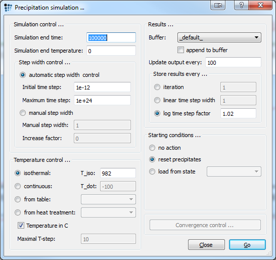
As the data gathered from the literature was taken at 1800F, which equals 982C, the precipitation simulation will be performed at this exact temperature. Check parameters below, then press Go! to start the simulation.
Plotting the results
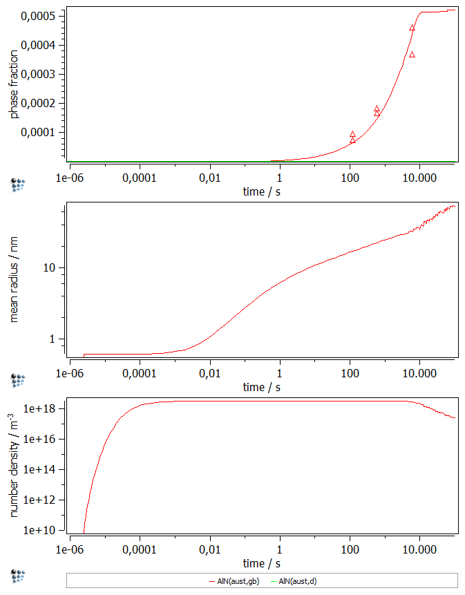
Create a new X-Y-Plot (p1) and add two new plots. Set a default x-axis to logarithmic with a scaling from 1e-6.. and label the axis time / s.
- Plot the phase fractions of the precipitates in the first figure (
f_prec$…) and the experimental data from the table. - Plot the mean radius of the precipitates in the second figure (
r_mean$…). - Plot the number density of the precipitates in the third figure (
num_part$…).
Label the y-axes accordingly.
Consecutive articles
This analysis is continued in the article AlN precipitation in ferrite.


