MatCalc version: 5.44.0017
Database: mc_fe.tdb, mc_x_FeAlCNNbTi.tdb
Author: E. Kozeschnik
Created: 2011-07-05
Revisions: G. Stechauner (2.11.2011 - Update for new version and database)

This example describes a strategy for evaluation of primary solidification microstructures based on purely thermodynamic grounds. This analysis can be utilized for a prediction of primary precipitation and microsegregation during casting. The results can serve as a basis for defining representative compositions in subsequent precipitation kinetics simulations of enriched and depleted regions in a (micro)segregated microstructure.

The example follows the analysis presented in ref.¹⁾.

Part I discusses the thermodynamic equilibrium analysis, which provides information on the expected phases occurring during cooling after solidification. It emphasizes the importance of composition sets in order to correctly capture complex miscibility gaps. The results of the equilibrium analysis are directly applicable for the correct setup of subsequent precipitation kinetics simulations.

1. E20-1 - Thermodynamic equilibrium analysis
2. E20-2 - Scheil-Gulliver analysis of primary precipitation
3. E20-3 - Accounting for the peritectic reaction
4. E20-4 - Scheil-Gulliver analysis of microsegregation
5. P20 - Precipitation simulation during continuous casting

Click here to view the script for this tutorial, and here to download the workspace file.

Consider a microalloyed steel during continuous casting. Even without employing kinetic simulation models, predictions can be made on the microsegregation state after solidification, the existence, type and amount of primary precipitates and equilibrium phases by simply employing thermodynamic equilibrium calculations. In the first part of this example, an analysis of equilibrium phases versus temperature is discussed in the presence of a miscibility gap for carbonitride precipitates. The following table summarizes the chemical composition of the steel used in this study. Nominal composition given in wt%.

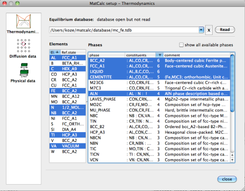
For simulation, either the 'mc_fe' or the 'mc_x_FeAlCNNbTi' database can be used, with the elements and phases selection as shown in the dialog below:

Open the database, select elements and phases, and read the database. Then enter the composition of the system in the 'Composition …' dialog of the 'Global' menu according to the table shown above.

Select 'Set start values' from the 'Calc' menu and evaluate equilibrium at 1000C. The output window contains the results, which should look like

#### /FCC_A1/ moles: 0.999136, gm: -62321.2 (-62321.2), sff: 0.990037 
Phasestatus: entered - active 
FE +9.89648e-01   C +9.85819e-03  AL +3.82546e-04   N +1.04746e-04 
NB +4.83777e-06  TI +1.83502e-06 

#### /FCC_A1#01/ moles: 0.000602176, gm: -124950 (-124950), sff: 0.50104 
Phasestatus: entered - active 
 C +4.89684e-01  NB +3.48361e-01  TI +1.52551e-01   N +9.27614e-03 
FE +1.28532e-04  AL +3.51584e-12 

#### /ALN/ moles: 0.000261912, gm: -188908 (178323), sff: 0.5 
Phasestatus: entered - active 
AL +5.00000e-01   N +5.00000e-01 

The equilibrium simulation shows that, at 1000C, austenite (fcc-Fe matrix) should be in equilibrium with AlN and a phase, which is denoted as FCC_A1#01, and which is a composition set of the FCC_A1 austenite.²⁾ The composition set phase FCC_A1#01 is a complex MX-type carbide, with a composition rich in Nb and C and containing additionally approximately 15% Ti.

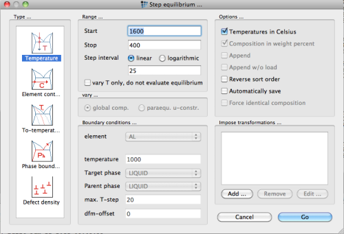
After calculation of an initial equilibrium, a stepped calculation is attempted next, with temperature as the independent variable. Open the 'Stepped calculation …' dialog from the 'Calc' menu and set the proper parameters with

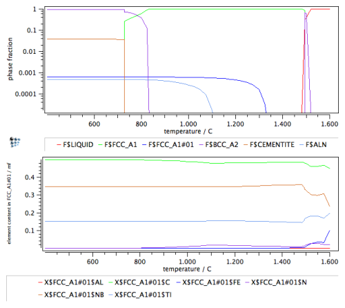
Perform the calculation, and display the results in a phase fraction versus temperature plot. Select 'X-Y-plot' from the 'Create new window …' dialog of the 'View' menu. Drag and drop the F$* variable into the window and enter T$C into the 'default x-data' item of the 'options' window. Select 'Use default-x axis' → 'yes', display the y-axis in log scale and label the axis. Finally, create a new plot (right mouse button → New plot) and drag and drop the composition of the FCC_A1#01 phase into the plot (X$FCC_A1#01$*). The plots then should look like

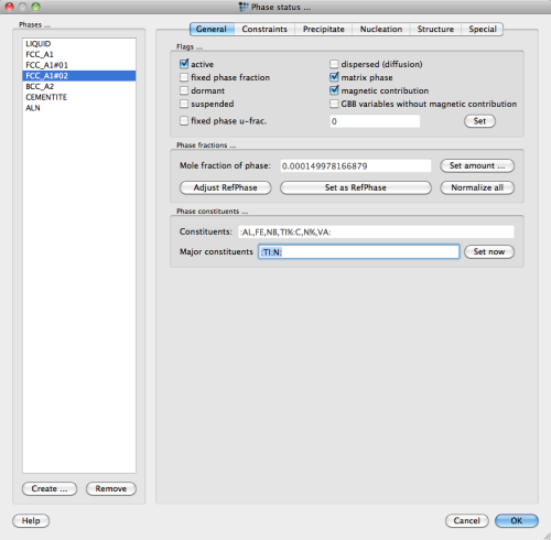
In Fe-based systems with micro-alloying additions of Nb-V-Ti and C-N, one often observes complex miscibility gaps between nitrides containing Ti (and sometimes Nb or V) and carbides containing Nb ( sometimes Ti and V). For the complex carbonitride FCC_A1#01, the enrichment of Ti and N in the otherwise Nb and C-rich phase suggests that a miscibility gap between the major constituent compositions NbC and TiN exists. In order to test this system behavior, an additional composition set for the complex carbonitride must be created from within the 'phase status' dialog and the major constituents of the two FCC_A1#01 and FCC_A1#02 phases must be set as :NB:C: and :TI:N: as shown for the latter phase in the dialog box below.

Note: After entering the new major constituents string, do not forget to press the 'Set now' button.

Calculate a new equilibrium at 1000C. The result should look like

#### /FCC_A1/ moles: 0.999245, gm: -62327.1 (-62327.1), sff: 0.989983 
Phasestatus: entered - active 
FE +9.89540e-01   C +9.92482e-03  AL +4.35383e-04   N +9.18718e-05 
NB +8.00257e-06  TI +2.01863e-07 

#### /FCC_A1#01/ moles: 0.000448713, gm: -118368 (-118368), sff: 0.50189 
Phasestatus: entered - active 
 C +4.91994e-01  NB +4.57005e-01  TI +4.46915e-02   N +6.11557e-03 
FE +1.93948e-04  AL +6.66924e-12 

#### /ALN/ moles: 0.000156233, gm: -188908 (178323), sff: 0.5 
Phasestatus: entered - active 
AL +5.00000e-01   N +5.00000e-01 

#### /FCC_A1#02/ moles: 0.000149978, gm: -202772 (-202772), sff: 0.500001 
Phasestatus: entered - active 
TI +4.89674e-01   N +4.56966e-01   C +4.30326e-02  NB +1.03194e-02 
FE +8.11633e-06  AL +5.51360e-16 

The simulation with the additional composition set now delivers an additional stable equilibrium phase, which is FCC_A1#02, and which is rich in Ti and N. Simultaneously, the Ti and N contents of the FCC_A1#01 phase are significantly reduced, since these elements have now partitioned mainly into the new phase.

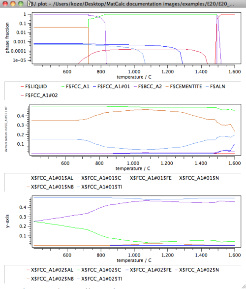
Finally, with the new phase set, the stepped calculation is repeated, with the results for the phase fractions and the composition of the two carbonitrides shown in the following diagram.

Note: If you cannot see the additional line for the phase fraction of the new composition set phase, make sure that you drag and drop the F$FCC_A1#02 variable into the first plot.

The new results now clearly distinguish between a TiN-rich carbonitride phase and a NbC-rich carbonitride phase, thus confirming the existence of a miscibility gap between the two phases. This results is an important indicator for appropriate phase selection in the precipitation kinetics simulation that will be attempted in the example P20 later.

Note: For an interpretation of the composition of the carbonitride phases, please consider the temperature stability range of the phases. For instance, the FCC_A1#02 phase is only stable in the temperature range of approximately 650 to 1450°C. The calculated compositions outside this range are corresponding to the hypothetical values that are evaluated by MatCalc according to the tangent construction for maximum driving force. These compositions are often unstable and show oscillations when evaluated farther outside the stability range. In these cases, the miscibility gap is unstable and should not be considered. The composition of the phases is then also not reliable and should not be considered.

Save the final results in workspace E20_1_equilibrium.mcw.

This analysis is continued in article Scheil-Gulliver analysis of primary precipitation