MatCalc version: 5.44.0003
Author: Georg Stechauner
Created: 2011-09-19
Revisions:

This example will build on the knowledge you got in part 1. If you haven't done part 1 by now, you should not continue here!

This example will continue where part 1 stopped, and generate a DSC signal for a full heat treatment. The performed steps will be:

• Quenching from liquid
• Heating to solution annealed temperature
• Quenching to RT
• Aging and subsequent cooling to RT

We will abstain from correcting the interface energy in the first part of this example. Later on, we will manipulate those values, to achieve the curve we measured in the labs. The simulated values will be compared to measured ones.

• TP20-1 - Simple cooling from above solution temperature
• TP20-2 - DSC signal during heating and cooling
• Techpaper on Multimodal size distribution of precipitates

Click here to view the script for this tutorial.

Consider the following Nickel-based alloy during the heat treatment we briefly discussed in the objectives. Mind that the chemical composition is given in wt%.

The first stable phase we will consider, is the LIQUID phase. As the LIQUID phase solidifies, FCC_A1 will become stable. During cooling, GAMMA_PRIME will precipitate. As we use the Heat Treatment GUI, you will have full control over the cooling rates. It is highly recommended, that you play around with different values, so you can see what happens!

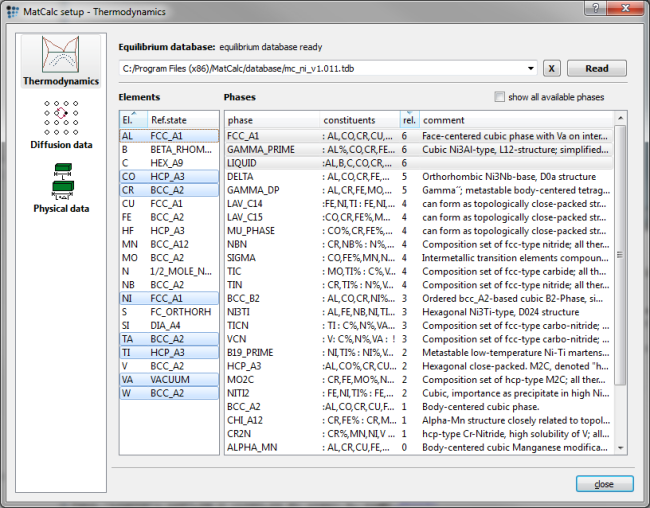
For simulation, the 'mc_ni' database, version 1.011, is used, with the elements and phases selection as shown in the dialog below:

Open the database, select elements and phases, and read the database. Then enter the composition of the system in the 'Composition …' dialog of the 'Global' menu according to the table shown above.

Next, read the diffusion database “mc_ni” (version 1.000 was used in this example).

In this example, we make use of some functions, which describe the temperature dependence of Young's modulus and the volumetric misfit parameter.

Open up the 'Variables & Functions' dialog and enter the following functions:

• Volumetric Misfit Parameter - misfit: ((-5.3e-13)*T$C^4+(6.43e-10)*T$C^3-(2.04e-7)*T$C^2-(9.29e-5)*T$C+0.632)/100
• Young's modulus, Matrix - y_modul_matrix: (-0.112*T$C+231.3)*1e9
• Young's modulus, Gamma_Prime - y_modul_gamP: (-0.052*T$C+189)*1e9

Open up the 'Precipitation domains …' dialog and create a new domain called 'ni-matrix '. Select FCC_A1 to be its matrix phase. Enter the following constants in the same dialog window to setup the microstructure:

• Grain diameter [m]: 500e-4
• Equilibrium dislocation density [m^-2]: 1e11
• Young's modulus matrix [Pa]: y_modul_matrix
• Subst. gb diffusion as ratio from matrix: 10^(11-0,005*T$C)
• Interst. gb diffusion as ratio from matrix: 10^(11-0,005*T$C)
• Subst. disl. diffusion as ratio from matrix: 10^(7-0.0025*T$C)
• Interst. disl. diffusion as ratio from matrix: 10^(7-0.0025*T$C)

Close this dialog window, and open the 'Phase status …' dialog. Create a Gamma_Prime precipitate with 40 size classes, attach it to the 'ni-matrix' domain and set the nucleation site to bulk; then set the following parameters:

• Young's modulus gamma_prime [Pa]: y_modul_gamP
• Volumetric misfit (dV/V): misfit (Make sure that the 'Account for coherent misfit stress' option is selected!)
• Coherency radius [m]: 30e-9

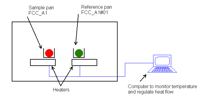
Next we have to generate a reference phase for the DSC curve (see figure above). To do so, open up the 'Phase status …' dialog window, and create an equilibrium phase for the FCC_A1 phase. Set the newly created FCC_A1#01 to 'fixed phase fraction', as we want the FCC_A1 to be the prevailing one, and calculate an equilibrium in the one phase field. Note how the chemical composition of both phases becomes identical!

Set the phase status of FCC_A1#01 to dormant, as we do not want it to change anymore. All the phases should be set now, and we can soon start the calculation!

Schauen, welche Plots und so wir brauchen, Text aus P1!

The next step of this example is to set up the plots, which will show us the phase fraction of Gamma_Prime_Precipitates, the DSC curve as well as the histogram showing the size of the precipitations.

Create a p1 plot, add a second plot. Change the default x-axis data to 'T$C' and rename it 'Temperature [°C]'. Make sure, you selected 'Yes' for using the x-axis on all plots. To plot the phase fraction of Gamma_Prime, we simply have to drag & drop the f_prec$gamma_prime_p0 to the first plot. Change title of plot and y-axis respectively.

The tricky part comes when plotting the DSC curve. As we cannot plot the heat flow with the given tools, we have to create a function on our own, to do so. Open the variables dialog once more, and add the following function to it:

• (HM$k-HMp$fcc_a1#01$k)/1000*(-50/60) (Discuss formula in detail!)

This function can now be found in the variables window. Add it to the second plot by dragging & dropping it. Derive the newly added series once and change the title and y-axis to DSC and heat flow [W/g] respectively.

To add the histogram, we need to add a p5 plot. When asked, select the Gamma_Prime_Precipitation. Then change the axes to logarithmic, change the factor on the x-axis to '1e9' as it will display the radius in [nm], and scale it to '0.1..'. Y-axis will show the number density in [m^-3], scale it to '10..'.

Move all windows to where you want them to be. Preferably in a way you can see the results.

Beschreiben und Screenshots von den Heat Treatment einstellungen Hinweisen darauf, hier selbst zu testen

Sagen das man Heat Treatment auswählen soll

Everything is set up, so let's get the calculation started!

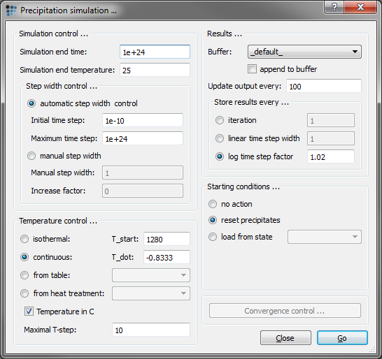
Open the 'Precipitation simulation …' dialog window and select continuous cooling. Enter the start and end temperature, as well as the desired cooling rate in the according dialog boxes. For the figure below, we used a starting temperature of 1280C, an end temperature of 25C, and a cooling rate of 50K/min (enter as -0.8333).Change the initial time step to 1e-10, as a lower value will result in a wrong, vertical line at the beginning. If your settings look like ours (check figure below), start the simulation.

Results aus P2 zeigen

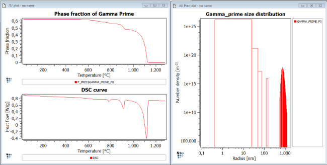
If all the prior steps were executed correctly, and the calculation finished without any errors, the below shown figures should be calculated.

We can see three peaks in the DSC curve. If you have a look at the buffer states, and go to the temperature of the first peak (~1110C), you can see the precipitation of mainly large, 1000nm big preciptates. Upon lowering the temperature, and reaching the second peak (~900C), a second population of smaller, 100nm in size precipitates can be seen. For temperatures below the last peak, a huge amount of the small, 1 to 10 nm in size precipitates form. This exact behavior can be measured experimentally and seen with TEM. For further information on the formation on multimodal precipitates, refer to Technical Paper .

We will continue in part 2, with simulating a full heat treatment, compared to only cooling in part 1. A comparison with real, experimental data will also be given.

This analysis is continued in article DSC signal during heating and cooling.